
View on GitHub

Open this notebook in GitHub to run it yourself
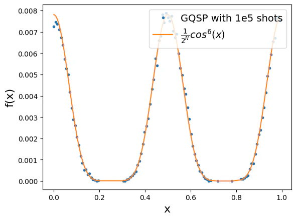
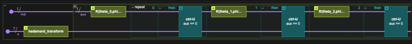
Generalized Quantum Signal Processing (GQSP) is a quantum algorithmic primitive that extends standard QSP, allowing one to block-encode arbitrary polynomials of unitary operations [1]. It removes the “realness” and parity restrictions on achievable polynomials that appear in QSP [2] and provides a simple recipe for constructing complex polynomials PP with P1|P|\le 1 on the unit circle. Moreover, it can be used to implement polynomials with negative powers, i.e., Laurent polynomials, further broadening the class of transformations accessible within this framework. The polynomial transformation is achieved by applying a sequence of arbitrary SU(2)\mathrm{SU}(2) rotations on an auxiliary qubit, rather than rotations in a fixed basis. The GQSP routine has several applications, such as state preparation and phase function transformations (eiH ⁣eif(H))(e^{iH}\!\to e^{if(H)}). A notable case is Hamiltonian simulation, where GQSP offers a more direct and flexible route compared to standard QSP.
  • Input: A unitary operator (quantum function) UU, and a target polynomial transformation P()P(\cdot) with P(x)1|P(x)| \le 1 for {xC:x=1}\{x \in \mathbb{C} : |x| = 1\}.
  • Output: A unitary that block-encodes P(U)P(U) using a single-qubit block variable.
Complexity: Applying a polynomial of degree dd requires dd controlled-UU calls and dd single-qubit SU(2)\mathrm{SU}(2) rotations.
Keywords: Quantum Signal Processing (QSP), Polynomial transformations, Block-encoding, Hamiltonian simulation, Phase functions.
In this demo we implement a simple instance of the GQSP primitive, preparing a state xcos3(x)\propto \sum_x\cos^3(x), by applying the corresponding polynomial on a diagonal unitary matrix. Using the gqsp quantum function from the open-library, phase assignment with phase, and utility classical function for obtaining the QSP angles, the implementation is done naturally.

!pip install -qq "classiq[qsp]"

Example: Preparing ψxcos3(x)x|\psi\rangle \propto \sum_x\cos^3(x)|x\rangle state

The idea of the algorithm is to prepare a diagonal unitary UU, such that Ux=eixxU|x\rangle = e^{ix}|x\rangle. Then, if we apply a polynomial P(x)P(x) such that P(eix)=cos3(x)P(e^{ix})=\cos^3(x), then we get P(U)x=cos3(x)P(U)|x\rangle = \cos^3(x). First, we write our function as a Laurent polynomial in eixe^{ix}: cos3(x)=18(eix+eix)3=18(e3ix+3eix+3eix+e3ix).\cos^3(x) = \frac{1}{8}(e^{ix}+e^{-ix})^3 =\frac{1}{8}(e^{3 ix}+3e^{ix}+3e^{-ix}+e^{-3ix}). Thus, the polynomial we are looking at is P(z)=18(z3+3z1+3z+z3)P(z) = \frac{1}{8}(z^{-3}+3z^{-1}+3z+z^3). First, we find the GQSP angles, by calling the gqsp_phases function. For numerical stability, we make sure the polynomial is strictly smaller than 1, by multiplying by a scaling constant.
import numpy as np

from classiq.applications.qsp import gqsp_phases

SCALING_CONST = 0.99

laurent_coeffs = 1 / 8 * np.array([1, 0, 3, 0, 3, 0, 1])
gqsp_phases = gqsp_phases(SCALING_CONST * laurent_coeffs)
The GQSP phases correspond to a polynomial with positive powers, P~(z)=18(1+3z2+3z4+z6)\tilde{P}(z) = \frac{1}{8}(1+3z^{2}+3z^4+z^6), however, the GQSP quantum function can shift it with a negative power, P(z)=zmP~(z)P(z) = z^{-m} \tilde{P}(z), with m=3m=3.
negative_power = 3
Next, we define the unitary we would like to operate on, Ux=eixxU|x\rangle = e^{ix}|x\rangle. It is simply defined by calling the phase function:
import numpy as np

from classiq import *


@qfunc
def u_func(x: QNum):
    phase(2 * np.pi * x)
Next, we define a model that prepares the desired state. This is done by initializing 012N/2x=02N1x|0\rangle\rightarrow \frac{1}{2^{N/2}}\sum^{2^N-1}_{x=0}|x\rangle, and then applying P(U)P(U) via gqsp.
NUM_QUBITS = 7


@qfunc
def main(x: Output[QNum[NUM_QUBITS, UNSIGNED, NUM_QUBITS]], ind: Output[QBit]):
    allocate(ind)
    allocate(x)
    hadamard_transform(x)
    gqsp(
        u=lambda: u_func(x), aux=ind, phases=gqsp_phases, negative_power=negative_power
    )
Now we can synthesize and execute the resulting quantum program
qprog = synthesize(main)
show(qprog)
Output:

Quantum program link: https://platform.classiq.io/circuit/3A4cHZmB5kCwN9E6dfDaU0unOrv
  

Screenshot 2025-09-14 at 10.53.11.png
NUM_SHOTS = 1e5
with ExecutionSession(qprog, ExecutionPreferences(num_shots=NUM_SHOTS)) as es:
    result = es.sample()
We can verify the resulting distribution against the expected one (recall that we need to post-select on the block variable ind==0)
import matplotlib.pyplot as plt

df = result.dataframe
df_post_selected = df[df.ind == 0].sort_values("x")
x, prob = df_post_selected.x, df_post_selected.probability
plt.plot(
    x,
    prob / SCALING_CONST**2,
    ".",
    label=f"GQSP with 1e{int(np.log10(NUM_SHOTS))} shots",
)
plt.plot(
    x,
    (1 / 2 ** (NUM_QUBITS / 2) * np.cos(2 * np.pi * x) ** 3) ** 2,
    "-",
    label=r"$\frac{1}{2^N}cos^6(x)$",
)
plt.xlabel("x", fontsize=16)
plt.ylabel("f(x)", fontsize=16)
plt.legend(loc="upper right", fontsize=14)
Output:
<matplotlib.legend.

Legend at 0x1266f4290>
  

output

References

[1]: Motlagh, D, and Nathan W. Generalized quantum signal processing. PRX Quantum 5 020368 (2024). [2]: Martyn JM, Rossi ZM, Tan AK, Chuang IL. Grand unification of quantum algorithms. PRX Quantum 2, 040203. (2021).