

View on GitHub
Open this notebook in GitHub to run it yourself
The HHL algorithm [1], named after Harrow, Hassidim and Lloyd, is a fundamental quantum algorithm designed to solve a set of linear equations:where is an matrix, and and are vectors of size . The algorithm prepares a quantum state that encodes the solution vector proportional to , starting from the input state . It achieves this by applying Quantum Phase Estimation (QPE) to extract the eigenvalues of , then performing a controlled rotation that effectively inverts these eigenvalues. The resulting amplitudes represent the solution state, which can be used to estimate properties of efficiently for certain classes of matrices.
The algorithm treats the problem in the following way:where , and is the desired precision. In comparison, the best classical method requires polynomial time (or for positive definite matrices). Therefore, the quantum algorithm apparently represents an exponential speedup in problem size; however, this speedup depends on strong assumptions: must be sparse, well-conditioned, and efficiently simulatable. Specifically, and should be (i.e., upper bounded by a polynomial expression with argument ). Moreover, should be loaded efficiently, and our goal is either to only estimate observables like quantities of the form , only sample or utilize for further matrix computations [6].Complexity: HHL can find a quantum representation of the solution in polylogarithmic time, with a runtime of roughly
- Input: A Hermitian matrix of size , normalized vector , and given precision .
- Promise: is Hermitian, sparse and well-conditioned. In addition, the eigenvalues of lie between and , where is the condition number of . The entries of vector can be loaded efficiently to a quantum state .
- Output: Solution vector encoded in the state , where: are eigenphases of a unitary , estimated up to binary digits and are coefficients in expansion of initial state into linear combination of eigenvectors of , such that . The solution vector allows one to efficiently estimate for a Hermitian matrix .
Solving linear equations appears in many research, engineering, and design fields. For example, many physical and financial models, from fluid dynamics to portfolio optimization, are described by partial differential equations, which are typically treated by numerical schemes, most of which are eventually transformed to a set of linear equations. For simplicity, the demo below treats a use case where the matrix has eigenvalues in the interval and . Generalizations to other use cases, including the case where and is not a Hermitian matrix or not of size , are discussed at the end of this notebook. The discussion begins with a concise overview of the algorithm, followed by its definition and implementation using Classiq’s built-in functions. We conclude by comparing the exact implementation of the algorithm with an approximate method, which is often more practical for real-world systems requiring extensive computational resources.
Keywords: Fundamental quantum algorithm, Exponential speedup, Linear equation solver
Algorithm Steps
The algorithm is composed of five main steps:- Three quantum variables, coined here a “memory”, “estimator” and indicator are initialized with , , and qubits respectively and the vector is encoded into the memory variable:
- Quantum Phase Estimation is applied to the initial state,
- Controlled rotations are applied to indicator bit with normalized constant ,
- Eigenvalues are uncomputed with QPE,
- Auxiliary bit value is measured: if is observed we obtain
Preliminaries
Defining Matrix of a Specific Problem
Output:
Define Hamiltonian
We next represent the Hamiltonian into the Pauli operators. This will allow evaluating , which is utilized in the Quantum Phase Estimation (QPE) stage and consequently, in the associated classiq function code block. Having the matrix or the Hamiltonian defined, the unitary operator can be created with theqpe_flexible function by passing in the unitary_with_power argument a callable function that applies a unitary operation raised to a given power.
The built-in function matrix_to_pauli_operator encodes the matrix into a sum of Pauli strings, which then allows to encode the unitary matrix with a product formula (Suzuki-Trotter).
This is a classical pre-processing that can be achieved by various decomposition methods, for example, you can compare with method described in [2].
The number of qubits is stored in the variable n.
Output:
How to Build the Algorithm with Classiq
The Quantum Part
The first step of the HHL algorithm involves loading the elements of the normalized RHS vector , into a quantum variable: where are the states in the computational basis. Below, we define the quantum functionload_b using the built-in function prepare_amplitudes.
This function loads the elements of amplitudes, which correspond to the entries of the vector , into the amplitudes of the state in the output variable memory.
Define HHL Quantum Function
Thehhl function performs steps 2-4 of the algorithm.
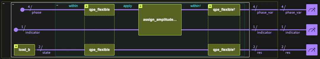
Steps 2 and 4 of the algorithm are achieved by applying the within_apply construct, where the within part corresponds to a flexible quantum phase estimation qpe_flexible.
The apply involves the controlled rotations of step 3, which are performed with assign_amplitude_table function.
The built in function qpe_flexible is given a function unitary_with_power which indicates how the powers are performed within the phase estimation procedure. In the following implementation, the powers are performed by Hamiltonian evolution, utilizing the hamiltonian_evolution_with_power function.
The normalization coefficient ensures the amplitudes are normalized.
Since eigenvalues of are normalized to be between and , the eigenvalues of the inverse matrix are between and . However, the amplitudes cannot surpass unity; we therefore choose as a lower bound of the minimum eigenvalue .
Arguments:
unitary_with_power: A callable function that applies a unitary operation raised to a powerk.precision: An integer representing the precision of the phase estimation process, (number ofestimatorqubits ).memory: An array representing the initial quantum state on which the matrix inversion is to be performed.estimator: Stores the estimation of the phase.indicator: An auxiliary qubit that stores the result of the inversion.
Set Execution Preferences
We prepare for the quantum program execution stage by providing execution details and constructing a representation of HHL model from a function defined in Quantum Modelling Language Qmod. The resulting circuit is executed on a statevector simulator. For other available Classiq simulated backends see Execution on Classiq simulators. To define this part of the model, we set the backend preferences by placingClassiqBackendPreferences with the backend name SIMULATOR_STATEVECTOR into the ExecutionPreferences.
The Classical Postprocess
After running the circuit a given number of times and collecting measurement results from the indicator and phase qubits we need to postprocess the data in order to find solution. Measurement values from circuit execution are denoted here byres_hhl.
Postselect Results
If all eigenvalues are -estimated (are represented by binary digits), then the uncomputation by inverse-QPE creates the state: If there is an error in step 3 and at least one eigenvalue is not -estimated, then after performing QPE, theestimator variable does not reset to .
This will further reduce the success probability of
In the general case, we postselect only states that return for indicator variable. In this tutorial, we will add another postselection condition on estimator variable, to return , in order to increase the accuracy of the solution result.
Note: Postselection can improve HHL algorithm results at the cost of more executions. In the future, when two-way quantum computing is utilized, postselection might be replaced by adjoint-state preparation, as envisioned by Jarek Duda [4].
The quantum_solution function defines a run over all the relevant strings holding the solution.
The solution vector will be inserted into the variable qsol, after normalizing with .
After the calculation we divide by to obtain the elements of .
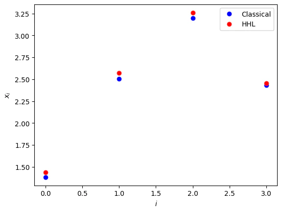
Compare Classical and Quantum Solutions
To compare between the quantum and classical solutions we first need to isolate the global phase of the quantum solution. Let the outcome state be , satisfying . We can isolate the phase by taking the scalar product of with , i.e., . We then evaluate , rotate by the appropriate angle, and take the real part. Note that only observables of the form (which are independent of the global phase) are accessible by a quantum experiment. The global phase is purely a numerical inconvenience which arises in the comparison the enteries classical solution with the quantum amplitudes and has no physical meaning in the implementation of the algorithm on actual hardware.Example: Implementation of with exact Hamiltonian Simulation
The phase estimation subroutine in the HHL algorithm involves a consecutive application of controlled powers of gates, i.e, conditional . In the present section, we implement these gates exactly and later compare the results to an approximate evaluation of these gates. While the implementation of exact Hamiltonian simulation provided here is not scalable for large systems due to the exponential growth in computational resources required, it serves as a valuable tool for debugging and studying small quantum systems. For sparse matrices, there is an efficient quantum algorithm for Hamiltonian simulation, see Ref. [7] and the technical notes section below.Synthesizing the Model (exact)
Output:
Statevector Simulation (exact)
Execute the quantum program. Recall that you chose a statevector simulator because you want the exact solution.Results (exact)
Output:

Example: Approximated Hamiltonian Evolution (Suzuki-Trotter)
The approximated Hamiltonian simulation is capable of handling larger and more complex systems, making it more suitable for real-world applications where exact solutions are computationally prohibitive. For the QPE we are going to use Classiq’ssuzuki-trotter function of order one for Hamiltonian evolution [3].
This function is an approximated one, where its repetitions parameter controls its error.
For a QPE algorithm with estimator size a series of controlled-unitaries with are applied, for each of which we would like to pass a different repetitions parameter depth (to keep a roughly same error, the repetitions for approximating is expected to be times the repetitions of ). In Classiq this can be done by working with a qpe_flexible, and passing a “rule” for how to exponentiate each step within the QPE in repetitions parameter.
R0 and REPS_SCALING_FACTOR dictate the number of repititions in the Suzuki-Trotter approximation.
The specific number of repititions depend on the Hamiltonian, and therefore, were chosen by trial and error.
For other examples, one would need to use different values for these parameters, please compare with specific example in Flexible QPE tutorial.
The relevant literature that discusses the errors of product formulas is available in Ref. [5].
Output:
Technical Notes
- The condition on the sparsity of arises from the following result, Ref. [7]: If is a Hermitian -spase matrix then one can implement an Hamiltonian simulation, up to error in the spectral norm with
- Before measurement we obtain the state
- We can replace the sparsity condition on by any restriction allowing efficient Hamiltonian simulation.
- The complexity of standard HHL algorithm is .
Generalizations
The use case treated above is a canonical one, assuming the following properties:- The RHS vector is normalized.
- The matrix is an Hermitian one.
- The matrix is of size .
- The eigenvalues of are in the range .
- Normalize and return the normalization factor
- Symmetrize the problem as follows:
- Complete the matrix dimension to the closest with an identity matrix and the vector will be completed with zeros.
- If the eigenvalues of are in the range you can employ transformations to the exponentiated matrix that enters into the Hamiltonian simulation, and then undo them for extracting the results: