Use this file to discover all available pages before exploring further.
View on GitHub
Open this notebook in GitHub to run it yourself
Quantum Phase Estimation (QPE) is a key algorithm in quantum computing, allowing you to estimate the eigenphase of a unitary matirx (or the eigenvalue of a Hermitian matrix).The algorithm is designed such that given the inputs of a Hermitian matrix M and an eigenvector ∣ψ⟩, the output obtained is θ, whereU∣ψ⟩=e2πiθ∣ψ⟩,U=e2πiM.By measuring the accumulated phase, the QPE algorithm calculates the eigenvalues relating to the chosen input vector. To read more about the QPE algorithm and its method for achieving the phase, refer to [1].Generally speaking, when the eigenvectors of the matrix are not known in advance yet the eigenvalues are sought, you can choose a random vector ∣v⟩ for the algorithm’s initial state.Some eigenvalues will be found as the vector can be described in the matrix’s basis, defined by the set of eigenvalues of M: {ψi}. Generally, any vector can be written as a superposition of any basis set, thus∣v⟩=∑iai∣ψi⟩andU∣v⟩=∑iaie2πiθi∣ψi⟩.Using execution with enough shots, you can obtain this set of θi; i.e., a subset of the matrix’s eigenvalues.This tutorial presents a generic usage of the QPE algorithm:
Define classical and quantum functions for constructing the algorithm.
Take a specific example, a matrix and some initial state.
Choose a resolution for the solution.
Find the related eigenvalues using QPE and analyze the results.
import mathimport numpy as npfrom classiq import *
As QPE obtains a phase in the form e2πiθ, there is meaning only for θ∈[−1/2,1/2). However, the matrix M can have any eigenvalue. To fix this discrepancy, the values of the matrix are rescaled. If
θ∈[λmin,λmax] you can use a normalization function to map those values into [−1/2,1/2).Perform the normalization procedure by:a.Defining the function get_normalization that finds a rough estimation for the eigenvalue with the largest absolute value.This yields a value \bar{\lambda} = {\max}\left\{|\lambda_\max|,|\lambda_\min|\right\}, such that you can assume θ∈[−λˉ,λˉ].b.Defining the function normalize_hamiltonian that normalizes by 2λˉ the Hamiltonian, and thus its eigenvalues, such that the evaluated span is then θ∈[−1/2,1/2].(Note that in this case θ=±1/2 correspond to the same phase, however, this is an edge case where the normalized Hamiltonian has exactly those two eigenvalues. To avoid this, you can apply an extra factor of (1−1/2m), where m is the size of the phase variable).
def get_normalization(hamiltonian): """ Bounds the eigenvalue with the maximal absolute value by summing all the absolute values of the Pauli coefficients """ abs_coeff = np.abs([term.coefficient for term in hamiltonian.terms]) return 2 * sum(abs_coeff)def normalize_hamiltonian(hamiltonian, normalization_coeff): return hamiltonian * (1 / normalization_coeff)
For QPE algorithms, the precision is set by phase register size m, such that the resolution is 1/2m. If the matrix needs to be normalized, the resolution will be distorted. In the case of normalization, the span of results for the QPE stretches between the lowest and highest possible phase, thus the resolution is mapped to ∼1/((λmax−λmin)∗2m).
Use the built-in qpe_flexible function, which allows you to prescribe the “telescopic” expansion of the powered unitary via the unitary_with_power “QCallable” (see Flexible QPE tutorial).Define two examples for the powered unitary:
Define the matrix to submit.This can be any Hermitian matrix with size 2n by 2n with n a positive integer.Throughout the code this matrix is given in the variable M.
Choose the vector that will be defined later as the initial condition for the run.There are two options: (1) define a random initial vector, or (2) choose some eigenvector of the matrix.For the demonstration, proceed with the first option:
np.random.seed(8)int_vec = np.random.rand(np.shape(M)[0])print("Your initial state is", int_vec)
Output:
Your initial state is [0.8734294 0.96854066 0.86919454 0.53085569]
Transform the matrix to ensure its eigenvalues are between −1/2 to 1/2.The QPE procedure is performed on the new normalized matrix.After the phases are obtained, gather the original phases of the pre-normalized matrix by performing opposite steps to this normalization procedure.
normalization_coeff = get_normalization(hamiltonian)new_hamiltonian = normalize_hamiltonian(hamiltonian, normalization_coeff)Mnew = M / normalization_coeff
Create a quantum model of the QPE algorithm using the Classiq platform with your desired constraints and preferences.Run two different models, with a unitary implementation, which is exact; or with an approximated prodcut formula.Synthesize the models and compare the resulting quantum programs.The exact version is a non-scalable approach, but a convenient one for small usecases.
print( f"Depth for QPE with exact Hamiltonian evolution: {qprog_exact.transpiled_circuit.depth}")print( f"Depth for QPE with approximated Hamiltonian evolution: {qprog_approx.transpiled_circuit.depth}")
Output:
Depth for QPE with exact Hamiltonian evolution: 384
  Depth for QPE with approximated Hamiltonian evolution: 6276
As expected, for this small usecase the exact evolution yeilds better results.Display it with the analyzer:
show(qprog_exact)
Output:
Quantum program link: https://platform.classiq.io/circuit/32pZjVUnGvgAFwr5Bve9w7vKFxB
Choose the number of eigenvalues to extract from the pool of results.The number_of_solutions value determines how many results are analyzed.Get the solution by multiplying back the normalization coefficient.
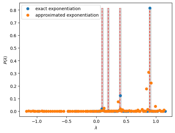
These are the results, including the error contributed from the resolution (the number of qubits participating in the QPE):
print( f"Your {number_of_solutions} solutions with the highest probability are:\n {solution_exact} (exact) \n {solution_approx} (approx)")energy_resolution = (1 / (2**n_qpe)) * 2 * normalization_coeffprint("the resolution of results is", energy_resolution)print("=" * 15 + " exact " + "=" * 15)for sol in solution_exact: print( "the solutions are between", sol - energy_resolution, "and", sol + energy_resolution, )print("=" * 15 + " approximated " + "=" * 15)for sol in solution_approx: print( "the solutions are between", sol - energy_resolution, "and", sol + energy_resolution, )
Output:
Your 2 solutions with the highest probability are:
   [0.8992759912499999, 0.40375656749999994] (exact)
   [0.8809234199999999, 0.9176285624999999] (approx)
  the resolution of results is 0.036705142499999996
  =============== exact ===============
  the solutions are between 0.8625708487499999 and 0.9359811337499999
  the solutions are between 0.36705142499999993 and 0.44046170999999995
  =============== approximated ===============
  the solutions are between 0.8442182774999999 and 0.9176285624999999
  the solutions are between 0.8809234199999999 and 0.9543337049999999