View on GitHub
Open this notebook in GitHub to run it yourself
Quantum Sawtooth Map and its Evolution
The system Hamiltonian
We start with the classical sawtooth map, written in terms of the action-angle variables where is the moment of inertia, and and are the kicking strength and kicking period, respectively. We now skip directly to the quantum model; the full derivation is provided in the Technical Notes at the end of this notebook. The derivation includes a straightforward quantization procedure, together with several redefinitions and normalizations. For the quantum map, we consider a finite Hilbert space of dimension , with momentum and position operators and defined by The Hamiltonian of the quantum sawtooth map reads: where is a dimensionless Planck constant (which can be related to the physical one by a factor of ). As part of the quantization procedure, the product is held constant. Consequently, the parameter controlling quantum effects is the Hilbert space dimension , with quantum fluctuations scaling as .The time evolution
A key practical advantage of quantum maps is the simplicity of their implementation on a quantum computer. Because the kicks are modeled as delta functions, the time-evolution operator factorizes into a sequence of evolutions generated by operators that are diagonal in complementary bases. In particular, for the sawtooth map considered in this notebook, the implementation does not require approximation overhead from product formulas or Chebyshev expansions, making it especially well suited for near-term quantum devices. The unitary evolution of the system between kick and , known as the Floquet operator, is given by: (This expression is exact and follows from modeling the kicks as delta-function impulses.) The evolution of the system from an initial state after kicks is therefore The kinetic term is diagonal in the momentum basis, while the kicking term is diagonal in the position basis. Since the two bases are related by a (discrete) Fourier transform, the Floquet operator can be efficiently simulated by alternating between these representations.Implementation in Qmod
We work with a Hilbert space of qubits, corresponding to a dimension . The time evolution of the model can be written in Qmod using only a few lines of code, taking advantage of the phase assignment construct.Dynamical Localization
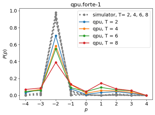
Depending on the non-dimensional parameters and , the quantum system exhibits different dynamical regimes and a variety of phenomena, such as dynamical localization, anomalous diffusion, and a positive quantum Lyapunov exponent. In this notebook we focus on the regime , in which dynamical localization can be observed (we refer to the literature, e.g., Ref. [1], for the full plethora of possible behaviors). For ,starting from a single excited momentum eigenstate , the wavefunction initially diffuses classically in momentum space, until quantum effects become relevant. This occurs at the Heisenberg time, defined as the time required to resolve the energy levels of the system. Beyond this time scale, quantum interference suppresses diffusion and leads to localization of the wavefunction over long times, with localization length . Since we consider a finite Hilbert space, localization persists only for a finite time and is observable provided that the localization length is smaller than the system size, . This condition is satisfied as long asExample: Localization in a 3 qubits System
We choose some hyper parameters, looking at a system on 3 qubits.Output:
Model definition
Defining a model with a parametric number of total time (number of kicks ):Output:

Output:
Execution
We execute the quantum program for different total numbers of kicks in order to examine the time evolution of the initial wavefunction.Output:
run_through_classiq.