View on GitHub
Open this notebook in GitHub to run it yourself
Part I — Theory and Framework
Background
Fluid dynamics are commonly well characterized by the famous Navier-Stokes equations - a set of non-linear coupled partial differential equations. Due to the non-linearity and multiscale nature of the dynamics, a precise solution for practical systems requires substantial numerical resources (for further details see the technical supplementary at the bottom). Instead of working directly with the macroscopic fluid equations, one can take a microscopic viewpoint: Fluids are modeled as collections of particles and their behavior is described statistically, using the Boltzmann transport equation. The solution to this equation gives the dynamics for the distribution of particles positions and velocities. A numerical approach for solving the kinetic PDE equation can be obtained by employing the (classical) Lattice Boltzmann Method (LBM).Lattice Boltzmann Method (LBM)
The Lattice Boltzmann Method simplifies the complex dynamics over the whole of phase space by replacing the velocity distribution with a discrete set of velocities, . Each lattice site is characterized by a -dimensional vector of distributions , representing the number of particles at that point with a velocity . The distributions evolve according to a discretized version of the Boltzmann transport equation under the Bhatnagar–Gross–Krook (BKG) approximation. Within the simplified description, the evolution is dictated by three distinct processes:- Streaming: distributions move along the velocity directions to neighboring lattice sites
- Collision: distribution of each site relaxes to equilibrium
Challenges in the classical approach
Despite the simplification, all classical solvers face several fundamental challenges:- The number of lattice sites required to accurately describe turbulence scales unfavorably. As a result, for realistic turbulence, the cost becomes prohibitive.
- Numerical instabilities can appear at high resolutions.
- For 3D systems of interest, the required number of lattice sites may be trillions.
Quantum Lattice Boltzmann Method
In the Quantum Lattice Boltzmann Method (QLBM) the distributions are encoded in the amplitudes of a quantum wavefunction , while the streaming, collision and reflections are achieved by application of unitary transformations. The template of QLBM algorithms is composed of three stages:- Initialization - the initial classical distributions and velocities are mapped to separate quantum variables.
- Evolution - repeated operatortion of propagates the state in time
Part II — Explicit Example: Collisionless Quantum Lattice Boltzmann Dynamics with Classiq
As a conceptual example, we consider a collisionless model in which the particle distribution evolves according to repeated streaming and reflection operations. We begin by defining the encoding of the initial distribution in the quantum register.State encoding
The set of classical states are encoded in quantum states of the form where the grid (, ) and velocity magnitude (, ) variables are encoded as QNum variables, and the velocity directions (, ) are encoded as single qubits. The QNums allow a straightforward implementation of shift operations, while the velocity directional encoding enables flipping the direction in the ‘th dimension by application of a single NOT operation on . For example, a quantum state means that there is a particle on lattice site with a left velocity of magnitude and down velocity of magnitude .Time evolution:
The time-step is composed of two operations:- Streaming: particles move one lattice site if their speed allows it (see below for further details).
- Reflection: particles hitting the obstacle are specularly reflected—direction is flipped and pushed back into the domain.

- Collisionless QLBM algorithm circuit.
Initial condition
The quantum state is initialized to be localized at a single grid point positioned to the left of the reflection obstacle. Velocities along the -axis are initialized uniformly, whereas along the -axis only non-negative velocities are sampled, uniformly distributed over their possible magnitudes.Observables
After running the quantum circuit, we measure the- spatial distribution - probability to find a particle at each site
- velocity distribution - propability over velocity magnitudes
Defining model hyperparameters
Scheduling function
A classical time-series function implements a Courant–Friedrichs–Lewy (CFL) counter, tracking the velocity magnitudes streamed at each time-step. The time steps duration are set such that at each step the distributions will at most transition to a neighboring lattice site. As a consequence, the durations generally vary between time-steps. Note, that in the following example represents a two dimensional vector. To evaluate the streamed velocities we first need to compute the time interval after the ‘th time-steps, . To this end, consider a distribution at a time-step at position , advancing with a speed away from a lattice site at . The fraction of the distance from the lattice site in the following time-step can be expressed as where is the lattice spacing. If particles may only travel to the nearest lattice site during a single time-step, to evaluate , we set , leading to . Finally, for multiple possible velocities, the limiting time step is evaluated by minimizing over all velocity magnitudes Utilizing we can evaluate for all velocites and determine which distributions have reached a lattice site.Initialization
Initializing the model parameters.Initial state preparation, setting parameters
We initialize the particles at a lattice point on the left-hand side of the lattice with a uniform velocity distribution in the y-direction and a non-negative uniform distribution in the x-direction.PhaseSpaceStruct:
Initiating model parameters and CFL schedule
The model is propagated formax_iters time-steps (each containing a streaming and reflection operation), and the reflecting object is placed between the corners of limits.
Schematic representation of the considered grid
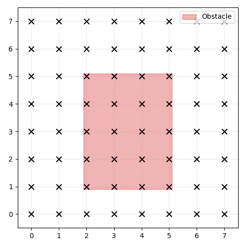
- Schematic representation of the analyzed example. An eight-by-eight grid, with a reflection object located in the center.
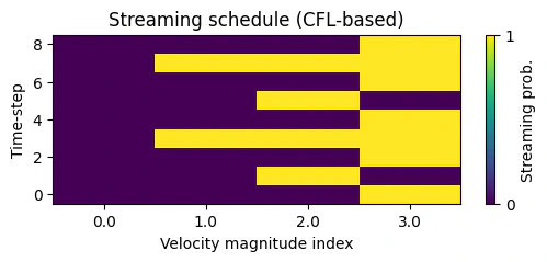
- Streaming schedule.
Streaming operator
The streaming operation propagates the particles based on theschedule, which contains the streamed velocity magnitudes at each time step.
Conditioned on whether the velocity magnitude appears in schedule[t], a sequential modular addition operation is performed on the associated grid variable .
The operation manifests a conditional translation of a specific set of positional states.
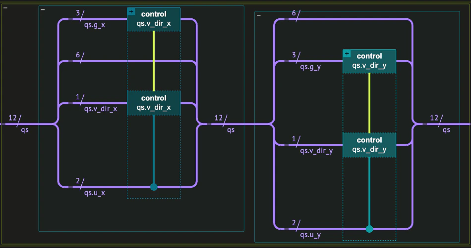
- Implementation of the streaming operator in Classiq
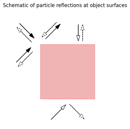
Specular Reflection
The boundary reflection operation effectively reflects particles that enter the boundaries. The boundary surfaces are assumed to be orthogonal to the lattice sites, and located right between two lattice sites. Each boundary surface is characterized by the lattice site inside the boundary closest to its surface,position, and the direction normal to the surface, direction.
Two types of reflections can occur:
(i) reflections from the corners of the reflecting object, and
(ii) reflections from the bulk of its surface.
(i) For particles colliding with a corner, the velocity components along both the and axes are reversed.
(ii) For particles colliding with the flat surface, only the velocity component normal to the surface is reversed, while the tangential component remains unchanged.
Such a reflection scheme enables modeling the reflection process without any ancillas.
This is achieved by ensuring that particles incident from different directions never scatter into the same outgoing direction.
Allowing multiple distinct incoming states to map onto a single outgoing state would correspond to a non-invertible transformation, thereby violating the unitarity condition required by the quantum circuit computation model.
A reflection operation is performed unitarily a controlled operations, effectively reversing the appropriate velocity of a particle colliding with the reflection object’s boundary.
The -component velocities of particles reaching the upper and lower surfaces of the rectangular object and -component, for particles reaching the left and right surfaces.
A reflection operation is implemented unitarily through controlled operations, effectively reversing the relevant velocity component of a particle upon collision with the boundary of the reflecting object. Specifically, the -component of velocity is reversed for particles striking the upper or lower surfaces, while the -component is reversed for those hitting the left or right surfaces. As a consequence, the velocity of particles reaching the corners is reversed.
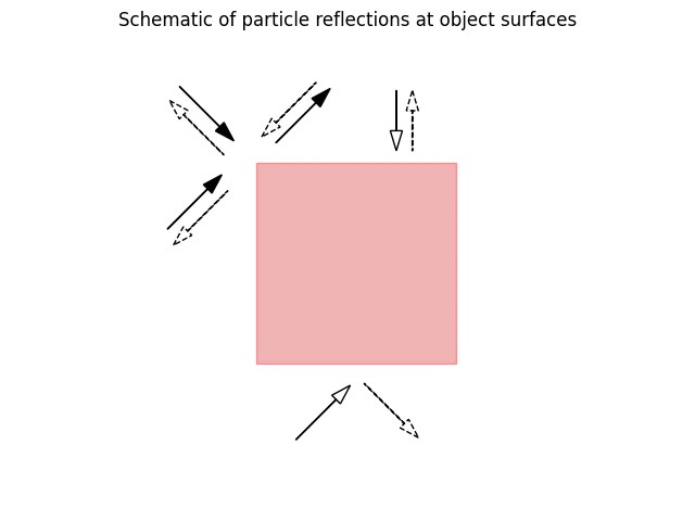
- Schematic representation of the reflection types.

- Implementation of the reflection operator within the main quantum circuit.
Building the quantum program
Execution and results
We run the quantum program on a statevector simulator to retrieve the full solution.| qs.g_x | qs.g_y | qs.v_dir_x | qs.v_dir_y | qs.u_x | qs.u_y | count | probability | bitstring | |
|---|---|---|---|---|---|---|---|---|---|
| 0 | 1 | 1 | 1 | 1 | 0 | 3 | 88 | 0.042969 | 110011001001 |
| 1 | 6 | 2 | 1 | 1 | 3 | 0 | 77 | 0.037598 | 001111010110 |
| 2 | 1 | 2 | 1 | 1 | 0 | 0 | 76 | 0.037109 | 000011010001 |
| 3 | 4 | 7 | 0 | 1 | 3 | 3 | 76 | 0.037109 | 111110111100 |
| 4 | 1 | 2 | 0 | 1 | 1 | 1 | 74 | 0.036133 | 010110010001 |
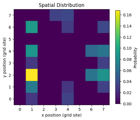
- Spatial distribution.
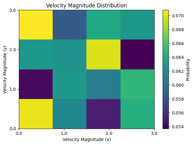
- Velocity magnitude distribution.
Analysis
The simulation starts with particles placed at lattice site , and their velocities are distributed uniformly — meaning each possible speed is equally likely at the beginning. We apply periodic boundary conditions, so particles that leave the domain on one side re-enter from the other. In addition, a reflecting obstacle is a rectangle with the corners situated at , , , and . As the system evolves, particles outside the obstacle move freely, while those reaching the obstacle bounce back. After several time steps, the particles cover the free space surrounding the reflecting object. The velocity-magnitude plot shows that all speeds still have roughly the same probability. This makes sense because no collisions occur in this setup, so the distribution of speeds doesn’t change over time, only the direction of the velocities. The small differences between probabilities come only from statistical fluctuations, since we are working with a finite number of samples from the quantum simulation.Part III
- Technical Background
Classical methods
The dynamics of fluids with low compressibility and isothermal conditions are described by the small Mach number limit of the Navier—Stokes equations: where is the velocity field, is the fluid density, is the hydrodynamic pressure, is the dynamic viscosity, and represents external body forces. The nonlinear and multiscale nature of these equations imposes substantial computational demands on classical solvers. For discretization-based approaches, the per-time-step computational complexity scales as where is the number of grid points per spatial dimension and is the dimensionality of the system. However, fully resolving all relevant turbulent scales requires a grid resolution that scales unfavorably with the Reynolds number, approximately as . Consequently, the overall computational cost of direct numerical simulation grows nearly exponentially with . The Reynolds number is a unitless quantity that measures the relative importance of inertial forces to viscous forces in a fluid flow. Turbulent flows correspond to high Reynolds numbers, where nonlinear interactions between scales dominate the dynamics. A further challenge lies in parallelization: enforcing incompressibility introduces global constraints that couple the velocity field across the entire domain, hindering the scalability of classical Navier–Stokes solvers and preventing fully local computation.Kinetic Formulation
An alternative, microscopic viewpoint is provided by the Boltzmann transport equation: where is the single-particle distribution function over phase space, represents external forces, and is the collision operator describing molecular interactions. The collision term involves a high-dimensional integral over all pre- and post-collision velocities and scattering angles, making its evaluation the dominant computational cost. For deterministic discretizations, the complexity per time step scales as where is the number of discrete velocity points per dimension.BGK Approximation
A major simplification is obtained by replacing the collision operator with a local relaxation term toward equilibrium: where is the relaxation rate and is the local Maxwellian equilibrium distribution. This Bhatnagar—Gross—Krook (BGK) approximation replaces the complex integral operator with a local operation that depends only on a few velocity moments. Despite this simplification, direct numerical integration of Eq.~(1) still requires evolving across both position and velocity grids, leading to a per-time-step complexity ofLattice Boltzmann Method (LBM)
The (LBM) offers an efficient and scalable alternative. LBM discretizes velocity space into a small set of representative directions, allowing collisions and streaming to be computed locally in time and space. This locality enables excellent parallelization and simplifies the handling of complex geometries and boundary conditions. The resulting per-time-step complexity scales as where is the number of discrete velocity directions per dimension (typically small and fixed).Figure codes
Figure 2
Figure 5