View on GitHub
Open this notebook in GitHub to run it yourself
Example
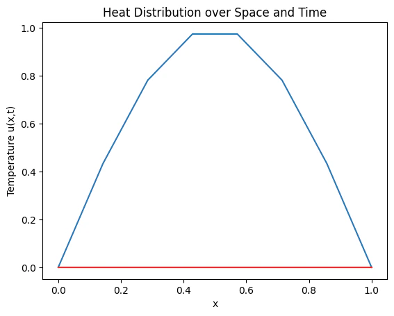
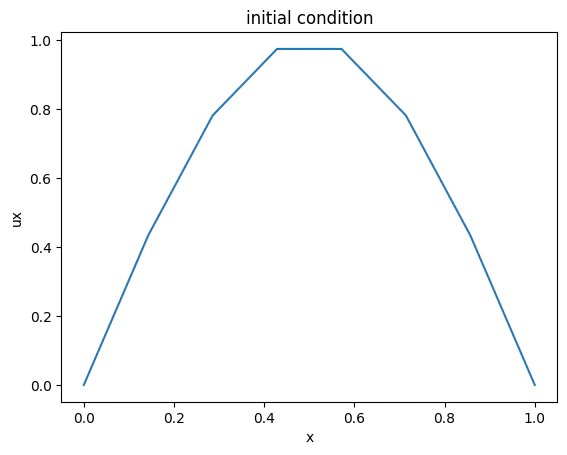
Let 1D stick of length L, the temperature distribution at time t = 0 (initial condition) and the temperature at the boundaries are constant and equal to 0 as formulated below:Initial Condition
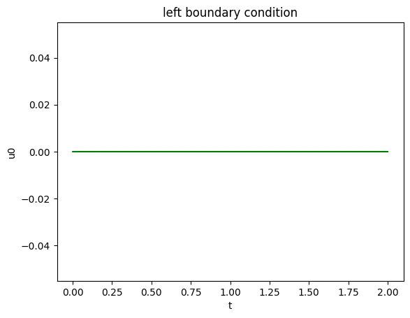
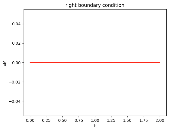
Boundary Conditions
- Left Boundary:
- Right Boundary:
Discretization of the Heat Equation
To solve the Heat Equation numerically, we discretize it using the finite difference method. In one spatial dimension: Substituting these into the Heat Equation gives: Rearranging terms, we obtain: This can be expressed in matrix form as: where is a matrix derived from the discretization, and represents the system’s state at the current time step. The goal is to compute , the state at the next time step.Matrix ( A ) and Vector ( b ): Discretization of the Heat Equation
To solve the 1D heat equation numerically, we discretize it using the finite difference method. The resulting system can be written as: where:- is the system matrix derived from the discretization of the second spatial derivative using a tri-diagonal structure.
- includes contributions from the initial conditions and boundary conditions.
Construction of Matrix ( L ):
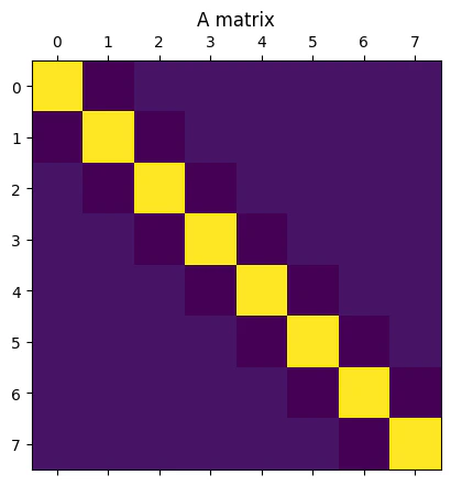
The Laplacian operator is represented as a tri-diagonal matrix: L = \begin\{bmatrix\} 2 & -1 & 0 & \cdots & 0 \\ -1 & 2 & -1 & \cdots & 0 \\ 0 & -1 & 2 & \cdots & 0 \\ \vdots & \vdots & \vdots & \ddots & -1 \\ 0 & 0 & 0 & -1 & 2 \end\{bmatrix\}Matrix ( A ):
Using the time step and spatial step , the system matrix is constructed as: where is the identity matrix.Visualization of Matrix ( A ):
The following code generates a matrix , constructs the vector for the initial and boundary conditions, and visualizes :- Initial Conditions:
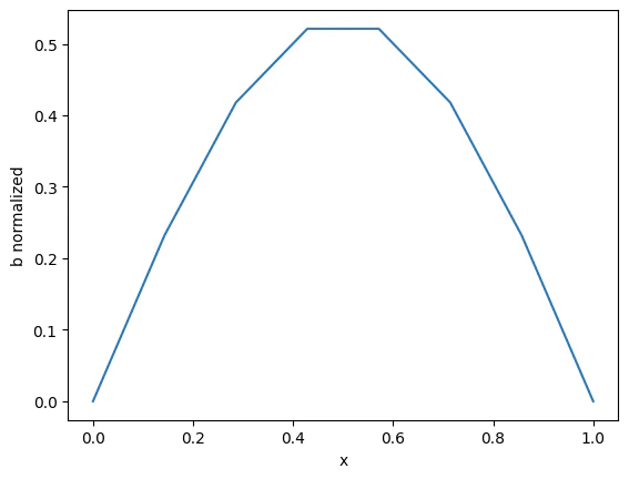
Output:
Output:
Problem formulation
is the vector representation of the temperature of the stick at time n. is the sum of the trmperature at time n-1 and boundary condition at time n. Problem operator define as the sum of Laplacian operator multiplied by discret operator and identity. So, we state the temperature at time n as a linear problem depends on time n-1 and the problem operator: Suppose we aim to predict the temperatue distribution at time n.-
Problem initialization:
- defined by initial condition.
- define as the sum of and the boundary condition.
-
Main loop:
for any i until n:
Block encoding
What is Quantum Block Encoding?
Quantum block encoding is a method in quantum computing used to embed a matrix or operator into a unitary matrix that can be implemented efficiently on a quantum computer. This technique is essential for quantum algorithms that require matrix operations, such as quantum machine learning, quantum linear algebra etc… THe starting point of QSVT is the availability of matrix A encoded as a block inside larger unitary operator U, when A is already unitary matrix BE become simply controlled-A.How to Block encode the matrix A of heat equation?
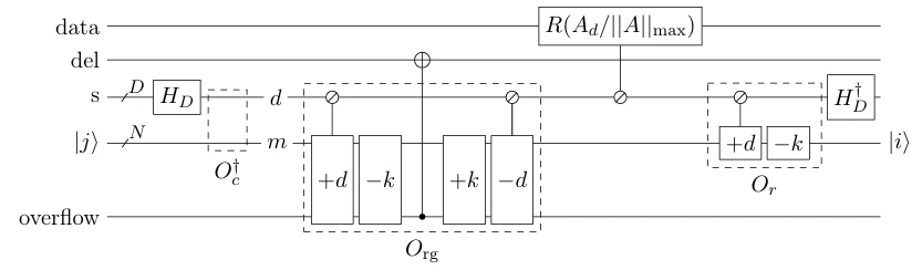
BE utilies the structure of the matrix A for building a quntum circuit representation (unitary operator) of matrix A. Condier matrix A has Toeplitz structure with D digonals, offset from the main diagonal by k: Specifically, A of our probles is Toeplitz matrix with 3 diagonals offset by k = 1: Lets set so matrix A is: Consider the mapping between (d,m) -> (i,j) where, (i,j) are the indices in matrix coordinates. (d,m) are the distinctiy and multiplicity of the values in A. i(d,m) = d - k + m. j(d,m) = m. Those mappings allows us to apply controlled rotation operator depending on the parameter d (superposition of posibilties of disdinct values), While m is simply the input state |j>The block encoding ciruit for Toeplitz matrix
Output:
Output:
Output:
Extracting the phases
In order to invert a matrix with QSVT we may cumpute classically the phases of QSP as in approximation to the the inversion function . Its done by computing the coefficients of the inversion matrix given the desierd accuracy and the lower bound of the smallest eigen value. The build-in function QuantumSignalProcessingPhases(..) takes the coefficient of descibed above and produces a list of phases that QSVT needed to be built.Output:
Quantum Singular Value Transformation (QSVT)
The Quantum Singular Value Transformation (QSVT) is a powerful quantum algorithm that manipulates the singular values of a matrix encoded in a quantum state. Starting by computing the QSP phases of the inersion function classically upon given accuracy, those phases are loaded to QSVT circuit desgined to manipulate the wigen values of matrix .Key Steps in QSVT:
- Block-Encoding:
- The matrix is embedded into a larger unitary matrix , preserving its singular values.
- This step ensures the matrix is compatible with quantum operations.
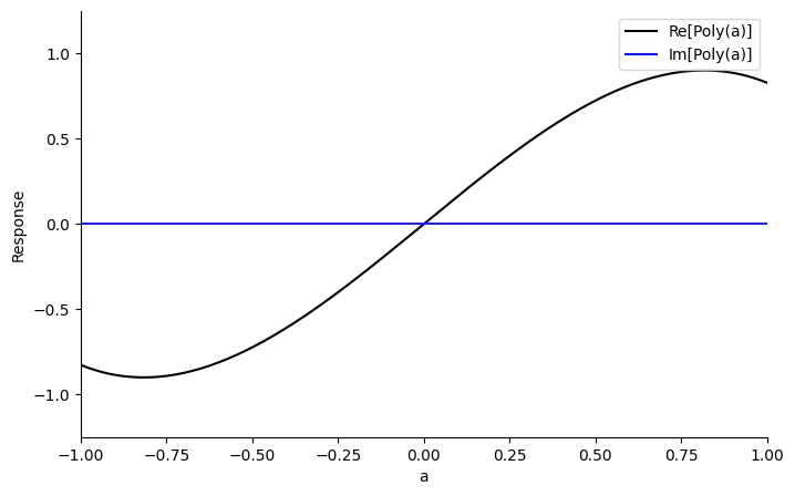
- Polynomial Approximation:
- QSVT applies a polynomial transformation to the singular values of .
- To solve , the polynomial is chosen as .
- Result Extraction:
- After applying QSVT, the solution is encoded in the quantum state.
- This state can be measured or further processed to extract the solution.
Implementation Plan:
- Construct the block-encoded unitary from the matrix .
- Design the QSVT circuit to apply .
- Execute the circuit using a quantum simulator and extract the solution.
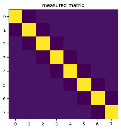
Results and Validation
problem formulation: is the vector representation of the temperature of the stick at time n. is the sum of the trmperature at time n-1 and boundary condition at time n. Problem operator define as the sum of Laplacian operator multiplied by discret operator and identity. So, we state the temperature at time n as a linear problem depends on time n-1 and the problem operator: Suppose we aim to predict the temperatue distribution at time n.-
Problem initialization:
- defined by initial condition.
- define as the sum of and the boundary condition.
-
Main loop:
for any i until n:
Output:
Output:
Output: