

View on GitHub
Open this notebook in GitHub to run it yourself
generate_pauli_list function, but the Pauli lists for 10 and 20 qubits (the examples in this notebook) have already been generated and cached in the glued_trees_cache.json file. However, if you would like to try recalculating the Pauli lists or calculating them for other qubit sizes, uncomment the line at the bottom of the code segment.
Output:
Quantum Algorithm
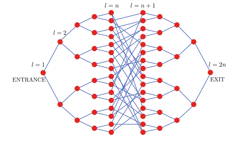
To model the columns of the glued trees structure as a system of coupled harmonic oscillators, we consider a matrix of size corresponding to the nodes of the glued trees structure, such that and is the number of columns of one of the two glued trees. This matrix is defined as , where is the adjacency matrix of the glued trees system using any ordering. For demonstration purposes, we use a simple linear ordering of this adjacency matrix such that the entrance node is first and the exit node is last. This matrix is symmetrical and takes the following shape: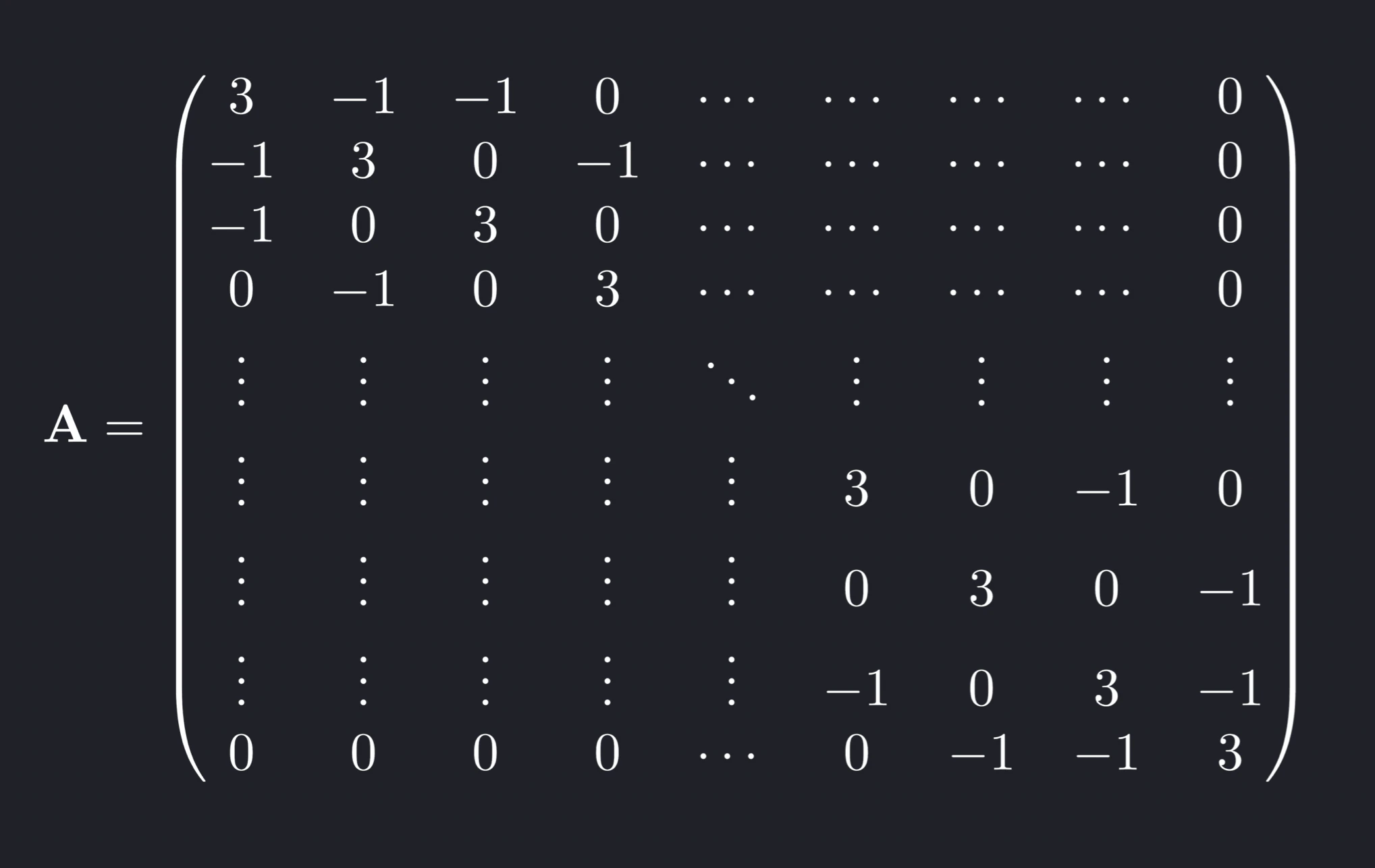
nx.adjacency_matrix function to generate an adjacency matrix using that ordering. We decompose using Cholesky decomposition to get a square matrix where its product with its conjugate transpose is equal to .
This matrix is the same size as , however, so we must pad it with four columns of zeroes to get our matrix of size so has a size corresponding to a power of two. We can then create the block Hamiltonian with the proper size using and , and generate its full Pauli list using the Classiq built-in matrix_to_hamiltonian function.
All Pauli list outputs are cropped so they have no more than 200 terms.
This is to ensure that the circuit depth is at a reasonable range (in the low thousands) given the limits of current quantum hardware. As a result of this approach, as the number of qubits increases, the accuracy of the Pauli list in comparison to the matrix it represents diminishes so the circuit depth remains roughly constant.
The Pauli list representation of for qubit sizes small enough to calculate (12 qubits and lower) are generated and cropped using the generate_pauli_list function, which uses an ad hoc approach that tries to represent the Pauli list as a whole as accurately as possible using only the 200 ostensibly most relevant terms to simulate the system.
The cropping algorithm, defined in the crop_pauli_list function, first selects 120 terms (60%) by going through each character position from the end to the start and picking the Pauli terms with the largest coefficients that contain each of the four possibilities (, , , ) at that character position. If all positions are exhausted before reaching 120 terms, the algorithm takes another pass through the character positions until 120 are selected.
The other 80 terms (40%) are selected by picking the 80 remaining terms with the largest coefficients.
The algorithm balances important high-coefficient terms with diversity in the 200 selected terms.
The Pauli lists for qubit sizes too large to fully calculate (greater than 12 qubits) are approximated by padding with the second character of the Pauli strings of the largest cropped Pauli list that can be generated in reasonable time, as this follows a pattern present in the vast majority of strings in the cropped Pauli list.
run_point.
This function takes in the number of qubits qubits and the time t to perform Hamiltonian simulation using the exponentiation_with_depth_constraint function in the Classiq software development kit.
The max_depth parameter is set to 1400, which is around the range of the current limit for comprehensible results in state-of-the-art quantum computers.
The num_shots parameter is set to 8192 to give enough room for significant spikes in a state to be apparent, given the high number of total possible states.
The resulting quantum state can be written as follows:
where and using a linear ordering of nodes.
Since the speed of the entrance node oscillator is represented by the quantum state and should have probability 1 at , there is no specific state preparation necessary for this system. It should also be noted that since our matrix is padded with four rows of zeroes, the highest four quantum states do not correspond to the displacement or speed of any oscillator.
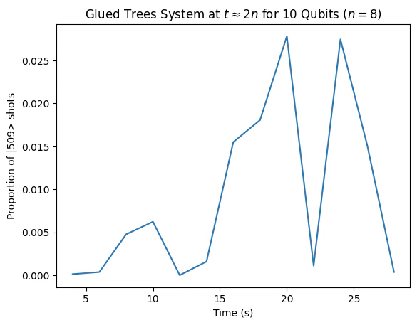
This means that the quantum state representing the speed of the exit node oscillator , which is what we are most interested in, corresponds to . We track this particular quantum state at time , expecting a spike that represents the system of oscillators “reaching” the exit node from the initial push to the entrance node.
We run the run_point function through a helper function run_range, which executes it 13 times in total for a given qubit size, spanning from to in two-second intervals.
This range gives time to observe oscillation occurring at the state value corresponding to while also being close enough around , the time where we expect a spike.
run_range for 10 qubits (), a higher qubit size that is still simulatable. In addition, it is low enough that its Pauli list can still be fully generated and cropped.
This instance of the function takes a few minutes to run. As defined, it uses the cached Pauli list for ten qubits in glued_trees_cache.json. To recalculate the Pauli list, ensure that you uncomment and run the two lines at the top of this notebook and add recalculate=True as the second parameter to the function:
Output:
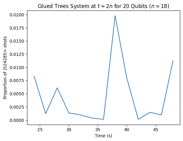
run_range for 20 qubits (), a qubit size that is still simulatable but whose Pauli list cannot be generated and is thus approximated using the Pauli list for 12 qubits.
This instance of the function takes a few minutes to run if the cached Pauli list is used.
Since this instance of the function requires generating the Pauli list for 12 qubits, which is very large, it takes much longer to run if you choose to recalculate the Pauli list.
You can also view the qmod file for the execution of run_point for 20 qubits at , which is saved in this directory as glued_trees_example.qmod:
Output:
results folder based on their qubit size.
The graph_results function creates a plot of the proportion of shots for the qubit state corresponding to for a given qubit size from to and saves it in the figures folder:
run_point function.
Perhaps the most interesting thing about the glued trees algorithm is that it is a relatively heavy case of using a quantum computer to gain an exponential advantage, usually requiring several executions at different time points to observe the intended result, but it can still execute effectively on present-day quantum hardware due to the Pauli list cropping. Suggestion: Try out the algorithm on both a simulator and quantum hardware for various qubit sizes.