Linear Combination of Hamiltonian Simulation (LCHS)

View on GitHub

Open this notebook in GitHub to run it yourself

The Linear Combination of Hamiltonian Simulation (LCHS) method [1] solves linear ODEs of the form $\frac{d}{dt}|u\rangle = -A|u\rangle$ on a quantum computer, where $A$ may be non-anti-Hermitian, leading to non-unitary time evolution. It works by expressing the propagator $e^{-At}$ as a continuous linear combination of unitary evolutions, which is then discretized and implemented using standard Hamiltonian simulation primitives.

Input:

A matrix $A = L + iH$ with $L \succeq 0$ (positive semidefinite) and $H = H^\dagger$ (Hermitian).

Block-encoding oracles for $H/\alpha_H$ and $L/\alpha_L$ .

The evolution time $t$ and target error $\epsilon$ .

Output: A quantum state proportional to $e^{-At}|u_0\rangle$ , obtained via post-selection on auxiliary qubits.

Complexity: The algorithm requires $\mathcal{O}(\alpha_A\, t \log(1/\epsilon))$ queries to the block-encoding oracle for $A$ [5], where $\alpha_A \geq \|A\|$ is the block-encoding normalization and $\epsilon$ is the target operator-norm error $\|e^{-At} - \tilde{U}\| \leq \epsilon$ . This is optimal in all parameters, improving the $\widetilde{O}(\alpha_A\, t \log^{1+o(1)}(1/\epsilon))$ scaling of prior work [1], [2].
Keywords: Non-unitary dynamics, Linear Differential Equations, Hamiltonian Simulation, Block Encoding, GQSP, Kernel Methods, Open Quantum Systems.

Background

The Problem

We wish to solve the linear ODE

\frac{d}{dt}|u\rangle = -A\,|u\rangle, \qquad |u(0)\rangle = |u_0\rangle,

where

A \in \mathbb{C}^{N \times N}

. When

A

is not anti-Hermitian, the solution

|u(t)\rangle = e^{-At}|u_0\rangle

is non-unitary and cannot be directly implemented as a quantum gate. We decompose

A = L + iH

where:

$H = \frac{1}{2i}(A - A^\dagger)$ is Hermitian (the conservative/oscillatory part),
$L = \frac{1}{2}(A + A^\dagger)$ is positive semidefinite (the dissipative/damping part).

Source terms. The homogeneous equation above can be extended to the inhomogeneous case

\frac{d}{dt}|u\rangle = -A|u\rangle + |b(t)\rangle

. Via Duhamel’s principle, the solution is

|u(t)\rangle = e^{-At}|u_0\rangle + \int_0^t e^{-A(t-s)}|b(s)\rangle\,ds.

Each term involves evaluating the non-unitary propagator

e^{-A\tau}

and can therefore be handled by LCHS. In practice, the integral is discretized using a quadrature rule, and each quadrature point contributes an additional LCHS call at the corresponding time

(t - s)

(see [5], Sec. 1.1.2 and [2]).

The LCHS Identity

The central insight of LCHS is the integral identity (Eq. 4 in [5], originally [1]):

e^{-At} = \frac{1}{\sqrt{2\pi}}\int_{-\infty}^{\infty} \hat{f}(k)\, e^{-i(kL + H)t}\, dk,

where

\hat{f}(k)

is the Fourier transform of a function

f

chosen to satisfy

f(x) = e^{-x}

for

x \geq 0

. For each

k \in \mathbb{R}

, the matrix

H + kL

is Hermitian, so the exponential

e^{-i(kL+H)t}

is a unitary operator that can be implemented using standard Hamiltonian simulation techniques. In practice this integral is truncated to a finite interval

[-R, R]

(where

R

is the truncation radius) and discretized into a finite sum that can be implemented via LCU on a quantum computer. A key innovation of [5] is the approximate LCHS: the kernel

f

need only approximate exponential decay (rather than match it exactly), which circumvents a no-go result from prior work and enables the optimal

O(\alpha_A\, t \log(1/\epsilon))

query complexity.

Kernel Function

Reference [5] uses the kernel function (Eq. 9, with

j=2

y=1

\hat{f}_2(k;\gamma,c) = \frac{2}{\sqrt{2\pi}} \frac{e^{c(1-ik)}\, e^{-(k^2+1)/(4\gamma^2)}}{1+k^2}.

This is a product of a Lorentzian

1/(1+k^2)

and a Gaussian

e^{-k^2/(4\gamma^2)}

. The Lorentzian alone is the Fourier transform of exact exponential decay

e^{-|x|}

, but its tails decay only as

1/k^2

, making it expensive to truncate the integral. The Gaussian envelope suppresses the tails exponentially, enabling truncation to a finite interval

[-R, R]

with small error. The tradeoff is that the kernel now only approximates exponential decay, with the approximation quality controlled by

\gamma

: larger

\gamma

gives a wider (flatter) Gaussian and a better approximation, at the cost of a larger truncation radius

R

. The shift parameter

c

controls the normalization factor

\alpha_{\hat{f}_2} \leq e^c

, which determines the post-selection success probability. Theorem 2 of [5] sets

\gamma = \frac{1}{c}\sqrt{c + \log\frac{1+1/(2\pi)}{\epsilon_{\mathrm{lchs}}}}

and

R = 2c\gamma^2

to guarantee kernel approximation error

\leq \epsilon_{\mathrm{lchs}}

Discretization

The integral is discretized on a uniform grid of

N = 2^J

points with spacing

h = 2R/N

over the interval

[-R, R)

([5], Theorem 3, which proves exponential convergence of the uniform quadrature):

e^{-At} \approx \frac{h}{\sqrt{2\pi}} \sum_{j=-N/2}^{N/2-1} \hat{f}_2(k_j)\, e^{-i(k_j L + H)t}, \qquad k_j = h \cdot j.

The stepsize

h

is chosen according to:

h \leq \frac{\pi}{\|L\| \cdot t/2 + \log\!\left(\frac{64\, e^{3c/2}}{15\,\epsilon_{\mathrm{disc}}}\right)},

The number of grid points

N = 2^J

is then

J = \lceil \log_2(2R/h) \rceil

. Note that a uniform quadrature is sufficient. This sum is implemented via LCU, with the kernel values

\hat{f}_2(k_j)

as coefficients.

Quantum Circuit Structure

The full LCHS quantum circuit consists of the following components:

Kernel state preparation: Load $|\hat{f}_2(k_j)|$ into an auxiliary register $|j\rangle$ .
Block-encoding of $H + k_j L$ : For each grid point $j$ , block-encode the Hermitian operator $(H + k_j L)/\alpha$ , where $\alpha = \alpha_L R + \alpha_H$ is the normalization.
Hamiltonian simulation: In this demo we apply the Jacobi-Anger polynomial approximation of $e^{-i(H+k_j L)\alpha t}$ using Generalized QSP on the walk operator derived from the block encoding.
Post-selection: Measure all auxiliary qubits in the $|0\rangle$ state to extract the desired output.

Preliminaries

import matplotlib.pyplot as plt
import numpy as np
import scipy.linalg as la

from classiq import *
from classiq.applications.qsp import (
    gqsp_phases,
    poly_jacobi_anger_degree,
    poly_jacobi_anger_exp_cos,
)
from classiq.qmod.symbolic import pi

Problem Definition and Parameters

We define the Hamiltonians

H

and

L

and derive all algorithm parameters — state size, block-encoding normalization, kernel shape, and error budget — from these operators and the desired precision.

H_PAULI = 0.5 * Pauli.X(0) * Pauli.X(1) + 0.5 * Pauli.Z(0) * Pauli.Z(1)
L_PAULI = 0.5 * Pauli.I(0) * Pauli.I(1) + 0.5 * Pauli.Z(0) * Pauli.I(1)

STATE_SIZE = H_PAULI.num_qubits
n_pauli_terms = max(len(H_PAULI.terms), len(L_PAULI.terms))
BLOCK_SIZE = max(1, int(np.ceil(np.log2(n_pauli_terms))))
alpha_H = sum(abs(t.coefficient) for t in H_PAULI.terms)
alpha_L = sum(abs(t.coefficient) for t in L_PAULI.terms)

T = 1  # evolution time

GQSP_EPS = 1e-5  # GQSP polynomial approximation error
LCHS_EPS = 1e-2  # LCHS kernel approximation error (Theorem 2 of [5])
DISC_EPS = 1e-2  # discretization / quadrature error (Theorem 3 of [5])
EPS = GQSP_EPS + LCHS_EPS + DISC_EPS

c = 2.0  # kernel shift (trades normalization e^c vs. integration range)

gamma = np.sqrt(c + np.log((1 + 1 / (2 * np.pi)) / LCHS_EPS)) / c
R = 2 * c * gamma**2  # truncation radius

h = np.pi / (
    alpha_L * T / 2 + np.log(64 * np.exp(3 * c / 2) / (15 * DISC_EPS))
)  # step size
J_SIZE = int(np.ceil(np.log2(2 * R / h)))
h = R / 2 ** (J_SIZE - 1)  # actual h after rounding to power-of-2 grid

alpha_tot = alpha_L * R + alpha_H

GQSP_SCALE_FACTOR = 0.99

print(f"Derived:  gamma={gamma:.4f}, R={R:.4f}, J_SIZE={J_SIZE}")
print(f"Errors:   GQSP_EPS={GQSP_EPS}, LCHS_EPS={LCHS_EPS}, DISC_EPS={DISC_EPS}")
print(f"          EPS (total) = {EPS}")

Output:

Derived:  gamma=1.2993, R=6.7529, J_SIZE=6
  Errors:   GQSP_EPS=1e-05, LCHS_EPS=0.01, DISC_EPS=0.01
            EPS (total) = 0.02001
  

Notice that in practice these bounds are worst-case and not tight, and the actual error is much smaller.

Classical Reference Simulation

Before building the quantum circuit, we implement the LCHS formula classically to verify correctness.

Exact: Direct matrix exponentiation $e^{-(L+iH)t}|u_0\rangle$ .
LCHS: The discretized sum $\frac{h}{\sqrt{2\pi}} \sum_j \hat{f}_2(k_j)\, e^{-i(H+k_jL)t}|u_0\rangle$ using exact matrix exponentials.

def signed_j_vals(J: int) -> np.ndarray:
    """Signed grid indices: -2^(J-1), ..., 2^(J-1)-1."""
    return np.arange(-(2 ** (J - 1)), 2 ** (J - 1), dtype=int)


def lchs_grid(R: float, J: int):
    """Compute the LCHS discretization grid."""
    N = 2**J
    h = 2 * R / N
    j = signed_j_vals(J)
    k = h * j
    return h, j, k


def kernel_fhat2(k: np.ndarray, gamma: float, c: float) -> np.ndarray:
    r"""Kernel function $\hat{f}_2(k;\gamma,c)$ from Eq. (6) of [5] with j=2, y=1."""
    k = np.asarray(k, dtype=float)
    return np.exp(-1j * k * c) / (1 + k**2) * np.exp(-(k**2 + 1) / (4 * gamma**2))

def truth_nonunitary(v0, L, H, t):
    """Exact non-unitary evolution: exp(-(L + iH)t) @ v0."""
    return la.expm(-(L + 1j * H) * t) @ v0


def lchs_classical(v0, L, H, t, *, R, J, gamma, c):
    """Discretized LCHS with exact matrix exponentials."""
    v0 = np.asarray(v0, dtype=complex)
    h, j, k = lchs_grid(R, J)
    w = kernel_fhat2(k, gamma=gamma, c=c)

    out = np.zeros_like(v0, dtype=complex)
    for kj, wj in zip(k, w):
        U = la.expm(-1j * (H + kj * L) * t)
        out += wj * (U @ v0)
    return out, h, k, w

Classical Verification

We verify the LCHS simulation against the exact solution using a random test problem.

def random_hermitian(M: int, *, seed=None, scale=1.0) -> np.ndarray:
    rng = np.random.default_rng(seed)
    A = rng.normal(size=(M, M)) + 1j * rng.normal(size=(M, M))
    H = (A + A.conj().T) / 2
    return scale * H


def random_psd(M: int, *, seed=None, rank=None, scale=1.0) -> np.ndarray:
    """Random positive semidefinite matrix via B^dag B."""
    rng = np.random.default_rng(seed)
    r = M if rank is None else int(rank)
    B = rng.normal(size=(r, M)) + 1j * rng.normal(size=(r, M))
    return scale * (B.conj().T @ B)


def fidelity(a: np.ndarray, b: np.ndarray) -> float:
    a, b = np.asarray(a, dtype=complex), np.asarray(b, dtype=complex)
    if np.linalg.norm(a) == 0 or np.linalg.norm(b) == 0:
        return 0.0
    a, b = a / np.linalg.norm(a), b / np.linalg.norm(b)
    return float(np.abs(np.vdot(a, b)) ** 2)

CLASSICAL_SIZE = 2**7

H_classical = random_hermitian(CLASSICAL_SIZE)
H_classical /= np.max(np.linalg.svd(H_classical, compute_uv=False))

L_classical = random_psd(CLASSICAL_SIZE)
L_classical /= np.max(np.linalg.svd(L_classical, compute_uv=False))

np.random.seed(1)
v0_classical = np.random.rand(CLASSICAL_SIZE).astype(complex)
v0_classical /= np.linalg.norm(v0_classical)

CLASSICAL_SIZE = 2**7

H_classical = random_hermitian(CLASSICAL_SIZE)
H_classical /= np.max(np.linalg.svd(H_classical, compute_uv=False))

L_classical = random_psd(CLASSICAL_SIZE)
L_classical /= np.max(np.linalg.svd(L_classical, compute_uv=False))

np.random.seed(1)
v0_classical = np.random.rand(CLASSICAL_SIZE).astype(complex)
v0_classical /= np.linalg.norm(v0_classical)

R_classical, J_classical = R, 6
t_classical = 10

out_exact = truth_nonunitary(v0_classical, L_classical, H_classical, t_classical)

out_lchs, *_ = lchs_classical(
    v0_classical,
    L_classical,
    H_classical,
    t_classical,
    R=R_classical,
    J=J_classical,
    gamma=gamma,
    c=c,
)

print(f"Fidelity (LCHS vs exact):  {fidelity(out_exact, out_lchs):.6f}")

Output:


Fidelity (LCHS vs exact):  1.000000

Quantum Implementation

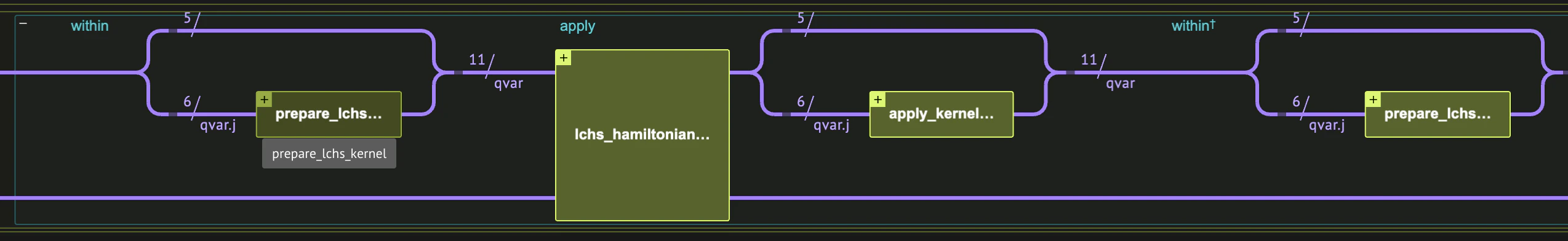
We now implement the full LCHS algorithm as a quantum circuit using Classiq. The circuit follows the structure described in the background:

Prepare the kernel amplitudes $|\hat{f}_2(k_j)|$ in the $|j\rangle$ register.
Block-encode the $j$ -dependent Hamiltonian $(H + k_j L)/\alpha$ .
Simulate the time evolution via GQSP on the walk operator.
Post-select on auxiliary qubits being $|0\rangle$ .

Data Structures

We define quantum struct types for the LCHS circuit. The LchsBlock struct holds the auxiliary registers:

j: a signed integer register for the grid index,
lcu_block: auxiliary qubit for the LCU of $H$ and $kL$ ,
linear_block: auxiliary qubit for the linear block-encoding of $k$ (explained below),
matrices_block: auxiliary qubits for the block-encoding of $H$ and $L$ .

class LchsBlock(QStruct):
    lcu_block: QBit
    linear_block: QBit
    matrices_block: QArray[BLOCK_SIZE]


class LchsVar(QStruct):
    x: QNum[STATE_SIZE]
    j: QNum[J_SIZE, SIGNED, 0]
    block: LchsBlock

Block-Encoding the Hamiltonians

For each grid point

j

, we need a block-encoding of the Hermitian operator

\frac{H + k_j L}{\alpha}, \qquad \alpha = \alpha_L R + \alpha_H.

This is achieved by an LCU decomposition:

\frac{H + k_j L}{\alpha} = \frac{\alpha_L R}{\alpha} \cdot \frac{k_j}{R} \cdot \frac{L}{\alpha_L} + \frac{\alpha_H}{\alpha} \cdot \frac{H}{\alpha_H}.

The factor

k_j / R

is block-encoded using a linear amplitude encoding:

|j\rangle|0\rangle \mapsto \frac{j}{2^{J-1}}|j\rangle|0\rangle + |\perp\rangle

, which embeds the linear function of

j

into an amplitude. The other constants are applied as part of the LCU probabilities. The Pauli-decomposed operators

H

and

L

(defined in the parameters cell above) are each block-encoded via lcu_pauli, which implements the LCU of Pauli terms using ancilla qubits.

@qfunc
def block_encode_H(x: QNum, block: QArray):
    lcu_pauli(H_PAULI * (1 / alpha_H), x, block)


@qfunc
def block_encode_L(x: QNum, block: QArray):
    lcu_pauli(L_PAULI * (1 / alpha_L), x, block)


@qfunc
def linear_be(x: QNum, ind: QBit):
    """
    Linear block-encoding: |j>|0> -> (j/2^(J-1))|j>|0> + |perp>.

Encodes the linear dependence on the grid index j.
    """
    assign_amplitude_table(
        amplitudes=lookup_table(lambda y: np.abs(y) / 2 ** (x.size - 1), x),
        index=x,
        indicator=ind,
    )
    X(ind)
    control(x < 0, lambda: phase(pi))


@qfunc
def block_encode_hamiltonians(qvar: LchsVar):
    """
    Block-encode sum_j |j><j| (h*j*L + H) / (R*alpha_L + alpha_H)
    using an LCU of the linear*L and H block-encodings.
    """
    lcu(
        [alpha_L * R, alpha_H],
        unitaries=[
            lambda: (
                linear_be(qvar.j, qvar.block.linear_block),
                block_encode_L(qvar.x, qvar.block.matrices_block),
            ),
            lambda: block_encode_H(qvar.x, qvar.block.matrices_block),
        ],
        block=qvar.block.lcu_block,
    )

Walk Operator and GQSP Hamiltonian Simulation

Given the block-encoding

U_A

(H + k_j L)/\alpha

, we construct the walk operator

W = (2|0\rangle\langle 0| - I) \cdot U_A

, whose eigenvalues are

e^{\pm i\arccos(\lambda_i/\alpha)}

for each eigenvalue

\lambda_i

(H + k_j L)

. We then use GQSP with a Jacobi-Anger polynomial approximation to implement

e^{-i\lambda_i t}

as a function of

\cos^{-1}(\lambda_i/\alpha)

, effectively realizing the Hamiltonian simulation

e^{-i(H + k_j L)t}

within the block.

@qfunc
def walk_operator(block_encoding: QCallable[LchsVar], qvar: LchsVar):
    """Walk operator: block_encoding followed by reflect-about-zero on the block."""
    block_encoding(qvar)
    reflect_about_zero(qvar.block)


@qfunc
def lchs_hamiltonian_simulation(qvar: LchsVar, aux: QBit, t: float):
    """
    Simulate exp(-i(H + k_j L) * t) for all j simultaneously using GQSP.

The effective time is alpha * t due to the block-encoding normalization.
    """
    t_effective = alpha_tot * t
    poly_degree = poly_jacobi_anger_degree(GQSP_EPS, t_effective)
    poly_exp_cos = GQSP_SCALE_FACTOR * poly_jacobi_anger_exp_cos(
        poly_degree, -t_effective
    )
    phases = gqsp_phases(poly_exp_cos)

    walk = lambda: walk_operator(block_encode_hamiltonians, qvar)

    gqsp(
        u=walk,
        aux=aux,
        phases=phases,
        negative_power=poly_degree,
    )

Kernel Preparation

The kernel state preparation loads the absolute values

|\hat{f}_2(k_j)|

into the

|j\rangle

e^{-ik_j c} = e^{-ihcj}

, is applied as a separate phase gate after the Hamiltonian simulation.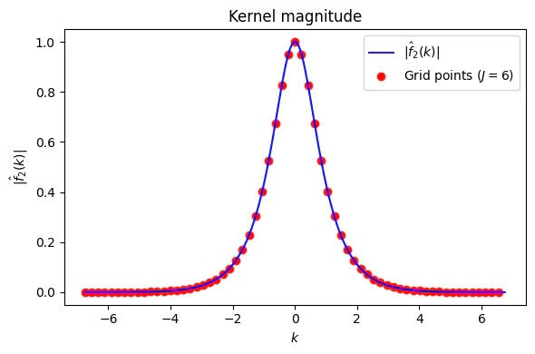

def kernel_func(k):
    """Absolute value of the kernel for state preparation."""
    return 1 / np.sqrt(1 + k**2) * np.exp(-(k**2) / (8 * gamma**2))


@qfunc
def prepare_lchs_kernel(x: QNum):
    """Prepare |f_hat_2(k_j)| into the j register."""
    amplitudes = lookup_table(lambda j: kernel_func(h * j), x)
    inplace_prepare_amplitudes(amplitudes, 0, x)


@qfunc
def apply_kernel_phase(j: QNum):
    """Apply the kernel phase e^{-i*h*c*j}."""
    phase(-h * c * j)

_, j_vals, k_vals = lchs_grid(R, J_SIZE)
fhat_vals = kernel_func(k_vals) ** 2

k_fine = np.linspace(-R, R, 500)
fhat_fine = kernel_func(k_fine) ** 2

plt.figure(figsize=(6, 4))
plt.plot(k_fine, np.abs(fhat_fine), "b-", linewidth=1.5, label=r"$|\hat{f}_2(k)|$")
plt.scatter(k_vals, np.abs(fhat_vals), c="r", label=f"Grid points ($J={J_SIZE}$)")
plt.xlabel("$k$")
plt.ylabel(r"$|\hat{f}_2(k)|$")
plt.title("Kernel magnitude")
plt.legend()
plt.tight_layout()
plt.show()

The full LCHS circuit wraps these steps in a within_apply pattern:

@qfunc
def lchs(qvar: LchsVar, aux: QBit, t: float):
    """Full LCHS routine: kernel preparation + Hamiltonian simulation + phase."""
    within_apply(
        lambda: prepare_lchs_kernel(qvar.j),
        lambda: [
            lchs_hamiltonian_simulation(qvar, aux, t),
            apply_kernel_phase(qvar.j),
        ],
    )

Running the Quantum Circuit

We define the main function, synthesize the circuit, and execute it using a statevector simulator. We post-select on the block register being

|0\rangle

to extract the LCHS output state.

np.random.seed(1)
v0 = np.random.rand(2**STATE_SIZE)
v0 /= np.linalg.norm(v0)


@qfunc
def initial_state_prep(x: QNum):
    inplace_prepare_amplitudes(v0, 0, x)


@qfunc
def main(x: Output[QNum[STATE_SIZE]], block: Output[QNum]):
    lchs_qvar = LchsVar()
    allocate(lchs_qvar)
    gqsp_aux = QBit()
    allocate(gqsp_aux)

    initial_state_prep(lchs_qvar.x)
    lchs(lchs_qvar, gqsp_aux, T)

    bind([lchs_qvar, gqsp_aux], [x, block])

qprog = synthesize(main)
show(qprog)

Output:

Quantum program link: https://platform.classiq.io/circuit/3CJZsTcki5NvhuXNzOIK9EgTVle
  

sv = calculate_state_vector(qprog)
post_selected = sv[sv.block == 0].sort_values("x")
q_out = post_selected.amplitude.values

display(post_selected)

Output:

Submitting job to simulator
  Job: https://platform.classiq.io/jobs/53c14875-06f8-4f2f-8811-8f544efd99f5
  

	x	amplitude	magnitude	phase	probability	bitstring
58	0	-0.009290+0.039227j	0.04	0.57π	0.001625	00000000000000
8	1	-0.162077-0.048177j	0.17	-0.91π	0.028590	00000000000001
40	2	-0.016073+0.054032j	0.06	0.59π	0.003178	00000000000010
29	3	-0.032474+0.071042j	0.08	0.64π	0.006101	00000000000011

Quantum vs.

Classical Comparison We compare the quantum LCHS output against:

Exact: Direct matrix exponentiation $e^{-(L+iH)t}|u_0\rangle$ .
LCHS (classical): Classical emulation of the quantum circuit (discretized LCHS with the GQSP polynomial approximation).

For this demonstration, we use the block-encodings defined above.

H_mat = pauli_operator_to_matrix(H_PAULI)
L_mat = pauli_operator_to_matrix(L_PAULI)
exact_out = truth_nonunitary(v0, L_mat, H_mat, T)

lchs_out, *_ = lchs_classical(
    v0,
    L_mat,
    H_mat,
    T,
    R=R,
    J=J_SIZE,
    gamma=gamma,
    c=c,
)

normalization = np.sqrt(post_selected.probability.sum())

print(f"Fidelity (quantum vs LCHS classical): {fidelity(q_out, lchs_out):.6f}")
print(f"Fidelity (quantum vs exact):          {fidelity(q_out, exact_out):.6f}")
print(f"Sub-normalization Factor (amplitude):   {normalization:.6f}")

assert np.isclose(fidelity(q_out, exact_out), 1, atol=EPS)

Output:

Fidelity (quantum vs LCHS classical): 1.000000
  Fidelity (quantum vs exact):          1.000000
  Sub-normalization Factor (amplitude):   0.198731
  

Technical Notes

Access model: The algorithm assumes block-encoding access to $H$ and $L$ separately. If only access to $A = L + iH$ is available, one can extract $H$ and $L$ via $H = \frac{1}{2i}(A - A^\dagger)$ and $L = \frac{1}{2}(A + A^\dagger)$ , though this may double the block-encoding cost. Alternatively, as noted in [5] (Sec. 1.1.5), one can block-encode $kL + H$ directly from a block-encoding of $A$ using the identity $kL + H = \frac{(k-i)A + ((k-i)A)^\dagger}{2}$ .
Time-dependent case: If $H$ or $L$ are time-dependent, the inner Hamiltonian simulation becomes time-dependent and can be handled using methods such as Dyson or Magnus series (see the Time Marching notebook).

The LCHS framework in [5] is stated in full generality for time-dependent

A(t)

Normalization and post-selection: The LCU of the kernel introduces a normalization factor $\alpha_{\hat{f}_2} = e^c \operatorname{erfc}(1/(2\gamma)) \leq e^c$ , which is $\Theta(1)$ for constant $c$ [5].

The final result is obtained by post-selecting on all block qubits being

|0\rangle

, with success probability determined by this normalization and the GQSP scaling factor.

Scalable kernel preparation: The inplace_prepare_amplitudes function used here loads arbitrary amplitudes but does not scale efficiently. [5] (Theorem 4) provides an efficient circuit for preparing the kernel state with $\mathcal{O}(\log(\|L\| + \log(1/\epsilon)) \log^{5/2}(1/\epsilon))$ two-qubit gates.

References

[1] An, D., Liu, J.-P., & Lin, L. Linear Combination of Hamiltonian Simulation for Nonunitary Dynamics with Optimal State Preparation Cost. Physical Review Letters 131, 150603 (2023). arXiv:2303.01029 [2] An, D., Childs, A. M., & Lin, L. Quantum algorithm for linear non-unitary dynamics with near-optimal dependence on all parameters. Communications in Mathematical Physics (2025). arXiv:2312.03916 [3] Motlagh, D. & Wiebe, N. Generalized Quantum Signal Processing. PRX Quantum 5, 020368 (2024). arXiv:2308.01501 [4] Hamiltonian Simulation with Block Encoding (Classiq Library) [5] Low, G. H. & Somma, R. D. Optimal quantum simulation of linear non-unitary dynamics. (2025). arXiv:2508.19238

Algorithms

Applications

Functions

Tutorials

Linear Combination of Hamiltonian Simulation (LCHS)

View on GitHub

Background

The Problem

The LCHS Identity

Kernel Function

Discretization

Quantum Circuit Structure

Preliminaries

Problem Definition and Parameters

Classical Reference Simulation

Classical Verification

Quantum Implementation

Data Structures

Block-Encoding the Hamiltonians

Walk Operator and GQSP Hamiltonian Simulation

Kernel Preparation

Running the Quantum Circuit

Quantum vs.

Technical Notes

References

Algorithms

Applications

Functions

Tutorials

View on GitHub

​Background

​The Problem

​The LCHS Identity

​Kernel Function

​Discretization

​Quantum Circuit Structure

​Preliminaries

​Problem Definition and Parameters

​Classical Reference Simulation

​Classical Verification

​Quantum Implementation

​Data Structures

​Block-Encoding the Hamiltonians

​Walk Operator and GQSP Hamiltonian Simulation

​Kernel Preparation

​Running the Quantum Circuit

​Quantum vs.

​Technical Notes

​References

Background

The Problem

The LCHS Identity

Kernel Function

Discretization

Quantum Circuit Structure

Preliminaries

Problem Definition and Parameters

Classical Reference Simulation

Classical Verification

Quantum Implementation

Data Structures

Block-Encoding the Hamiltonians

Walk Operator and GQSP Hamiltonian Simulation

Kernel Preparation

Running the Quantum Circuit

Quantum vs.

Technical Notes

References