Solving Elliptic Curve Discrete Logarithm Problem with Shor's Algorithm

View on GitHub

Open this notebook in GitHub to run it yourself

Introduction and Problem Statement

The Elliptic Curve Discrete Logarithm Problem (ECDLP) is a fundamental cryptographic challenge that underlies the security of elliptic curve cryptography (ECC). While classical algorithms require exponential time to solve ECDLP, Shor’s quantum algorithm can solve it efficiently in polynomial time.

Elliptic Curve Definition

An elliptic curve is a special type of mathematical curve defined by a cubic equation. For our purposes, we can think of it as the set of points

(x, y)

that satisfy the Weierstrass equation:

E : y^2 = x^3 + ax + b

where

a

and

b

are constants that define the specific shape of the curve. Key Properties:

Smooth curve: The curve has no sharp corners, breaks, or self-intersections (this requires $4a^3 + 27b^2 \neq 0$ )
Symmetric: The curve is symmetric about the x-axis - if $(x, y)$ is on the curve, then $(x, -y)$ is also on the curve
Point at infinity: We add a special “point at infinity” denoted $\mathcal{O}$ that serves as the identity element for point addition , as will be explained in the next section.

Cryptographic Context: For cryptographic applications like Bitcoin’s digital signatures, we work with elliptic curves over finite fields

\mathbb{F}_p

where

p

is a large prime number. Instead of the smooth curves we might visualize over real numbers, we get a discrete set of points:

E(\mathbb{F}_p) = \{(x, y) \in \mathbb{F}_p \times \mathbb{F}_p \mid y^2 = x^3 + ax + b\} \cup \{\mathcal{O}\}

The crucial property for cryptography is that these points form a group under a special addition operation. This means:

You can “add” any two points on the curve to get another point on the curve
There’s an identity element ( $\mathcal{O}$ ) where $P + \mathcal{O} = P$ for any point $P$
Every point has an inverse
Addition is associative: $(P + Q) + R = P + (Q + R)$

How Elliptic Curve Point Addition Works

The elliptic curve “addition” operation geometric interpretation: To add two points

P

and

Q

on the curve, draw a straight line through them. This line will intersect the elliptic curve at exactly one more point

R'

. The sum

P + Q

is then defined as the reflection of

R'

across the x-axis.

Figure 1: Visualized representation of the addition operation on the elliptic curve $y^2 = x^3 - 5x + 6$ over the real field. Algebraic Process: This geometric process translates into explicit coordinate formulas:

Calculate a slope $\lambda$ based on the input points
Use $\lambda$ to compute the x-coordinate of the result: $x_3 = \lambda^2 - x_1 - x_2$
Use $\lambda$ and $x_3$ to compute the y-coordinate: $y_3 = \lambda(x_1 - x_3) - y_1$

Elliptic Curve Addition Cases: In general, elliptic curve point addition must handle several cases:

Generic case: Two distinct points $P \neq Q$ where $P \neq -Q$

Slope: $\lambda = \frac{y_Q - y_P}{x_Q - x_P} \pmod{p}$

Point doubling: Adding a point to itself $P + P$

Slope: $\lambda = \frac{3x_P^2 + a}{2y_P} \pmod{p}$

Inverse points: $P + (-P) = \mathcal{O}$ (point at infinity)
Adding point at infinity: $P + \mathcal{O} = P$

Group Property: This addition rule ensures that the sum of any two points on the curve is always another point on the curve, maintaining the group property essential.

The Elliptic Curve Discrete Logarithm Problem (ECDLP)

Formally, an instance of the Elliptic Curve Discrete Logarithm Problem (ECDLP) is defined as follows: Let

G \in E(\mathbb{F}_p)

be a fixed and publicly known generator of a cyclic subgroup of

E(\mathbb{F}_p)

with known order

\text{ord}(G) = r

.Let

P \in \langle G \rangle

be a fixed and publicly known element in the subgroup generated by

G

. The problem is to find the unique integer $l \in \{1, 2, \ldots, r\}$ , called the discrete logarithm, such that $P = l \cdot G$ .

Why “Logarithm” for Point Addition? The term “discrete logarithm” might seem confusing at first in the context of elliptic curves, since the group operation here is point addition, not multiplication. However, the elliptic curve discrete logarithm problem (ECDLP) is a special case of the general discrete logarithm problem (DLP) (see the “discrete log” notebook), where the group happens to be defined by elliptic curve point addition rather than modular multiplication. In the Discrete Logarithm Problem, the group operation is modular multiplication, and exponentiation refers to repeated multiplication . In the elliptic curve setting, the scalar multiplication

l \cdot G

refers to adding the point

G

to itself

l

times. Below is a comparison of the two settings:

	Discrete Logarithm Problem (DLP)	Elliptic Curve DLP (ECDLP)
Group operation	Modular multiplication	Modular point addition
Expression	Modular exponentiation: $g^l = h$	Modular scalar multiplication: $l \cdot G = P_{target}$
Goal	Find $l$ given $g$ and $h$	Find $l$ given $G$ and $P_{target}$

In both cases:

A generator element ( $g$ or $G$ ) is known
A target element ( $h$ or $P_{target}$ ) is known
The task is to find the exponent or scalar $l$ such that the group operation applied to the generator yields the target

The term “logarithm” is used by analogy: just as logarithms solve for exponents in multiplicative groups, the discrete logarithm solves for the scalar in additive or elliptic curve groups.

Real-World Impact and Applications

Cryptographic Applications:

Digital Signatures: Power cryptocurrency systems like Bitcoin and Ethereum, enabling secure ownership proofs without revealing private keys
TLS/SSL Certificates: Use ECC-based key exchange (e.g., ECDHE) to secure HTTPS traffic across the internet
Mobile Communications: Employ protocols such as ECDSA and ECIES for device authentication and secure messaging in 4G/5G networks
Lightweight Cryptography: ECC is well-suited for resource-constrained environments, and is used in protocols like DTLS and TLS-PSK for IoT security
Secure Messaging and Encryption Standards: ECC forms the basis of cryptographic protocols in standards like Suite B, used in high-security communications

Why ECC is Preferred Over RSA: Elliptic curve cryptography offers the same security as RSA but with much smaller key sizes:

ECC-256 provides security equivalent to RSA-3072
Smaller keys mean faster computations and less storage
Critical for resource-constrained devices like smartphones and IoT sensors

Our Specific Example $E(\mathbb{F}_7)$

We’ll work with a concrete example on a small finite field to demonstrate the concepts, following the approach outlined in Roetteler et al. [1]. Our specific example will demonstrate elliptic curve operations over points

(x, y) \in \mathbb{F}_7 \times \mathbb{F}_7

: Elliptic Curve:

y^2 = x^3 + 5x + 4 \pmod{7}

Problem: Find the discrete logarithm

l

such that:

l \cdot G = P_{target}

Where:

Generator point $G = [0, 5]$
Target point $P_{target} = [0, 2]$

This means we need to find how many times we must add

G

to itself to get

P_{target}

. Solution:

l = 4

, since

4 \cdot [0, 5] = [0, 2]

Let’s verify by computing the multiples of

G = [0, 5]

$1 \cdot G = [0, 5]$
$2 \cdot G = [0, 5] + [0, 5] = [2, 1]$ (point doubling)
$3 \cdot G = [2, 1] + [0, 5] = [2, 6]$
$4 \cdot G = [2, 6] + [0, 5] = [0, 2]$ ✓

Therefore,

l = 4

is indeed the discrete logarithm we’re seeking. Curve Properties The elliptic curve

y^2 = x^3 + 5x + 4 \pmod{7}

contains the following points:

$[0, 2], [0, 5], [2, 1], [2, 6], [3, 2], [3, 5], [4, 2], [4, 5], [5, 0]$
Plus the point at infinity $\mathcal{O}$

Generator $G = [0, 5]$ properties:

Multiples: $1 \cdot G = [0, 5]$ , $2 \cdot G = [2, 1]$ , $3 \cdot G = [2, 6]$ , $4 \cdot G = [0, 2]$ , $5 \cdot G = \mathcal{O}$
Order: $r=5$ (since $5 \cdot G = \mathcal{O}$ )

Note: The order $r$ is the smallest positive integer such that $r \cdot G = \mathcal{O}$ (point at infinity).

# Define our elliptic curve and problem parameters
class EllipticCurve:
    def __init__(self, p, a, b):
        """
        Represents an elliptic curve of the form y^2 = x^3 + a*x + b (mod p)
        """
        self.p = p
        self.a = a
        self.b = b

    def __repr__(self):
        return f"EllipticCurve(p={self.p}, a={self.a}, b={self.b})"


# Problem parameters for our specific ECDLP instance
CURVE = EllipticCurve(p=7, a=5, b=4)
GENERATOR_G = [0, 5]
GENERATOR_ORDER = 5
INITIAL_POINT = [4, 2]
TARGET_POINT = [0, 2]

Shor’s Algorithm for ECDLP

Shor’s quantum algorithm [2] provides an efficient way to solve the discrete logarithm problem that would be intractable for classical computers. The algorithm proceeds as follows:

Algorithm Overview

Superposition Preparation: Create two quantum registers in a superposition of all possible integers between 0 and a large number
Periodic Function Evaluation: Apply a periodic function that takes the two registers as input and computes the output in an auxiliary register
Period Extraction: Apply an inverse Quantum Fourier Transform to reveal the hidden period of the function

Shor’s algorithm for solving the ECDLP is analogous to Shor’s algorithm for integer factorization. Both prepare large superpositions of inputs, feed them to a periodic function, and exploit the QFT routine to reveal hidden periodicities that allow efficient computation of the discrete logarithm (see the “discrete log” notebook).

The Periodic Function for Elliptic Curve

The key function evaluated in quantum superposition is:

f(x_1, x_2) = x_1 \cdot G - x_2 \cdot P_{target} = (x_1 - x_2 \cdot l) \cdot G

where the last equality holds by the definition of the discrete logarithm

l

(since

P_{target} = l \cdot G

). The function

f

exhibits periodicity in both variables:

\forall r, \quad f(x_1 + r \cdot l, x_2 + r) = f(x_1, x_2)

where

r

is the order of the generator

G

. When the quantum measurement finds inputs where

f(x_1, x_2) = \mathcal{O}

, the quantum Fourier transform extracts this period structure, revealing relationships that allow us to solve for the discrete logarithm

l

. In our quantum implementation, we actually evaluate $P_0 + x_1 \cdot G - x_2 \cdot P_{target}$ where $P_0$ serves as an auxiliary starting point that doesn’t affect the final discrete logarithm but helps avoid certain edge cases in the quantum arithmetic.

Quantum Oracle Function Implementation

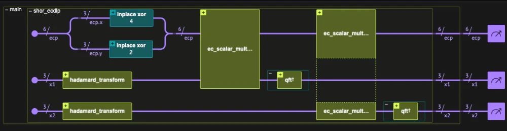
The core of our implementation is the shor_ecdlp quantum function that orchestrates the entire algorithm. It implements the function

|x_1\rangle|x_2\rangle|0\rangle \rightarrow |x_1\rangle|x_2\rangle| P_0 + x_1 \cdot G - x_2 \cdot P_{target}\rangle.

Expected Quantum Flow

Initialization : All variables start in $|0\rangle$ state
State Preparation : Set initial elliptic curve point
Superposition Creation : Apply transformation to create superposition over the possible values of $x_1$ and $x_2$
Quantum Arithmetic : Perform elliptic curve computation $P_0 + x_1 \cdot G - x_2 \cdot P_{target}$ in superposition
Period Extraction : Apply inverse QFT to extract period information

Quantum Struct Approach: We use a QStruct called EllipticCurvePoint to group the x and y coordinates together, making the code more organized and mathematically intuitive. Quantum Variables:

Variable	Purpose
`x1`	First quantum register for period finding (ranges 0-7)
`x2`	Second quantum register for period finding (ranges 0-7)
`ecp`	Quantum elliptic curve point during computation

Classical Parameters:

Variable	Purpose
`P_0`	Starting point
`G`	Generator point
`P_target`	Target point

*Note: In this case the order is not a power of

So instead of creating the entire uniform distribution on the x1, x2 variables, we load them with the uniform superposition of only the first #GENERATOR_ORDER states (see the “discrete log” notebook for more examples).*

We do that using the prepare_uniform_trimmed_state library function, which efficiently prepares such a state.

from classiq import *
from classiq.qmod.symbolic import ceiling, log


class EllipticCurvePoint(QStruct):
    x: QNum[CURVE.p.bit_length()]
    y: QNum[CURVE.p.bit_length()]


@qfunc
def shor_ecdlp(
    x1: Output[QNum],  # first quantum variable for period finding
    x2: Output[QNum],  # second quantum variable for period finding
    ecp: Output[
        EllipticCurvePoint
    ],  # third quantum variable for elliptic curve point coordinates
    P_0: list[int],  # starting point - classical
    G: list[int],  # generator point - classical
    P_target: list[int],  # target point - classical
) -> None:
    """
    Main quantum function implementing Shor's algorithm for ECDLP.
    """
    # Step 1: Allocate quantum resources to variables
    var_len = GENERATOR_ORDER.bit_length()
    allocate(var_len, False, var_len, x1)
    allocate(var_len, False, var_len, x2)

    # Step 2: Initialize ecp to P_0
    allocate(ecp)
    ecp.x ^= P_0[0]
    ecp.y ^= P_0[1]

    # Step 3: Create superposition on x1 and x2
    hadamard_transform(x1)
    hadamard_transform(x2)

    # Step 4: Quantum elliptic curve arithmetic in superposition
    # First: ecp = P_0 + x1·G
    ec_scalar_mult_add(ecp, x1, G, CURVE.p, CURVE.a, CURVE.b)

    # Second: ecp = P_0 + x1·G - x2·P_target
    neg_target = [P_target[0], (-P_target[1]) % CURVE.p]
    ec_scalar_mult_add(ecp, x2, neg_target, CURVE.p, CURVE.a, CURVE.b)

    # Step 5: Inverse Quantum Fourier Transform for period extraction
    invert(lambda: qft(x1))
    invert(lambda: qft(x2))

Quantum Elliptic Curve Addition

Algorithm Hierarchy Overview

The shor_ecdlp function orchestrates Shor’s algorithm, but its computational core is the ec_scalar_mult_add function, which performs quantum scalar multiplication in superposition. This function computes the expression

P_0 + k \cdot G

where

k

is in quantum superposition, enabling the algorithm to evaluate all possible scalar values simultaneously.

Quantum Scalar Multiplication (`ec_scalar_mult_add`)

Our implementation uses an efficient hybrid classical-quantum approach. We precompute all the powers-of-two multiples of the base point

P

classically:

P, 2P, 4P, 8P, \ldots, 2^{n-1}P

. Then we compute the scalar multiple using controlled additions of these precomputed points following the binary representation of the scalar. Algorithm: For scalar

k = \sum_{i=0}^{n-1} k_i 2^i

with

k_i \in \{0, 1\}

k \cdot P = \sum_{i=0}^{n-1} k_i 2^i P = \sum_{i=0}^{n-1} k_i (2^i P)

Implementation Steps:

Classical Preprocessing: Compute powers $P, 2P, 4P, \ldots$ classically
Quantum Control: For each bit $k_i$ , perform controlled addition of $2^i P$ to the accumulator

When

k

is in superposition

|k\rangle

, all possible scalar values are processed simultaneously:

|k\rangle|(x,y)\rangle \rightarrow |k\rangle|(x,y) + k \cdot P\rangle

All doubling operations happen classically through the ell_double_classical function, leaving only controlled point additions for the in-place elliptic curve point addition quantum function ec_point_add.

@qperm
def ec_scalar_mult_add(
    ecp: EllipticCurvePoint,  # elliptic curve point
    k: QArray[QBit],  # scalar in binary representation (LSB to MSB)
    P: list[int],  # classical point to multiply [x, y]
    p: int,  # prime modulus
    a: int,
    b: int,  # curve parameters
) -> None:
    """
    Quantum scalar multiplication: computes k*P and adds to ecp in-place.
    """
    n = k.size  # Number of bits in scalar k
    current_power = P.copy()  # Start with 1·P = P
    # Process each bit of k from LSB (bit 0) to MSB (bit n-1)
    for i in range(n):
        # Controlled point addition: if k[i] = 1, add current_power to accumulator
        control(k[i], lambda: ec_point_add(ecp, current_power, p))
        # Classical update for next iteration: current_power = 2 * current_power
        if i < n - 1:  # Don't double after the last iteration
            curve = EllipticCurve(p=p, a=a, b=b)
            current_power = ell_double_classical(current_power, curve)

Classical Point Doubling (`ell_double_classical`)

The doubling of the classically known generator is implemented as follows:

def ell_double_classical(P, curve):
    """
    Classical elliptic curve point doubling for updating powers in ec_scalar_mult_add.

Returns 2P for a point P on the elliptic curve.
    """
    p = curve.p
    x, y = P
    # Slope calculation: s = (3*x² + a) / (2*y) mod p
    numerator = (3 * (x * x % p) + curve.a) % p
    denominator = (2 * y) % p
    s = (numerator * pow(denominator, -1, p)) % p
    # x-coordinate of the result
    xr = (s * s - 2 * x) % p
    # y-coordinate of the result
    yr = (y - s * ((x - xr) % p)) % p
    # Return the result, with y in the standard form
    return [xr, (p - yr) % p]

Quantum Point Addition (`ec_point_add`)

The ec_point_add function performs the fundamental operation of adding two elliptic curve points in a quantum-reversible manner. Our Implementation Simplification: Following the approach in [1], our implementation focuses only on the generic case where the two points are distinct, not inverses of each other, and neither is the neutral element. These exceptional cases are rare (for large

p

) , except when the accumulation register is initialized to the neutral element. Note: *To avoid edge cases (as described above) through the entire quantum scalar multiplication, we chose to initialize the accumulation elliptic curve point with a non-zero point (

P_0 = [4, 2]

) rather than the neutral element. This strategy does not affect the measurement statistics after the Quantum Fourier Transform, since it only adds a global phase to the final quantum state. We deliberately selected a starting point that lies on the elliptic curve but is not within the subgroup generated by

G

. Additionally, we exploited the fact that the order of

G

is not a power of 2* Disclaimer: This is an engineered example chosen to allow simulation of a small model where edge cases effect the results. In general, such an initialization is not always possible. Algorithm Overview (Generic Case Only):

Input: Quantum point $(x_1, y_1)$ and classical point $G = (G_x, G_y)$
Slope calculation: Compute $\lambda = \frac{y_1 - G_y}{x_1 - G_x} \pmod{p}$ using quantum modular inverse
Result coordinates:

$x_{result}:= x_3 = \lambda^2 - x_1 - G_x \pmod{p}$
$y_{result}:= y_3 = \lambda(x_1 - x_3) - y_1 \pmod{p}$

Cleanup: Uncompute auxiliary values to maintain reversibility

Reference: The ec_point_add function is based on Algorithm 1 from “Quantum resource estimates for computing elliptic curve discrete logarithms” by Roetteler et al. (2017) [1] To implement ec_point_add, we need a complete library of reversible modular arithmetic operations which we import directly from the Classiq open library.

Modular Arithmetic Functions imported from Classiq Open Library

Organized by Category:

Basic Modular Operations:

modular_add_inplace
Modular addition
modular_negate_inplace
Modular negation
modular_subtract_inplace
Modular subtraction

Constant Operations:

modular_add_constant_inplace
Modular addition of a classical constant

Multiplication Operations:

modular_multiply
Modular multiplication
modular_square
Modular squaring

In our example, we will first implement modular inversion using a mock quantum function mock_modular_inverse based on a classical lookup table specifically for modulo 7, instead of implementing the full quantum modular inversion function modular_inverse_inplace (based on “Kaliski’s algorithm”), which requires significant qubit resources. *The above choice is driven by the practical desire to first fully simulate the entire elliptic curve discrete logarithm (ECDLP) algorithm flow within the limits of currently available quantum simulators. The full ECDLP synthesized circuit (including the full modular_inverse_inplace implementation) is presented at the end of this notebook.*

import math

from classiq.qmod.symbolic import subscript


@qperm
def mock_modular_inverse(x: Const[QNum], result: QNum, modulus: int) -> None:
    """
    Performs the transformation |x>|0> → |x>|x^(-1) mod modulus> for x in 1..modulus-

1. This is a mock implementation using controlled operations based on lookup table values.
    If the modular inverse does not exist, sets the 2nd register to 

0.
    """
    # Generate the lookup table for modular inverses
    inverse_table = lookup_table(
        lambda _x: pow(_x, -1, modulus) if math.gcd(_x, modulus) == 1 else 0, x
    )
    result ^= subscript(inverse_table, x)

@qperm
def ec_point_add(
    ecp: EllipticCurvePoint,
    G: list[int],  # Classical point coordinates [Gx, Gy] on the curve
    p: int,  # Prime modulus
) -> None:
    """
    Performs in-place elliptic curve point addition of a point whose coordinates are
    stored in quantum struct object and a classically known point.
    """

    n = CURVE.p.bit_length()
    slope = QNum()  # aux quantum register for lambda (slope)
    allocate(n, slope)
    t0 = QNum()  # aux quantum register for internal arithmetic
    allocate(n, t0)

    # Extract classical coordinates
    Gx = G[0]  # x2
    Gy = G[1]  # y2

    # Step 1: # y <-- (y1 - y2) mod p
    modular_add_constant_inplace(p, (-Gy) % p, ecp.y)

    # Step 2: # x <-- (x1 - x2) mod p
    modular_add_constant_inplace(p, (-Gx) % p, ecp.x)

    # Step 3: # λ <-- (y1 - y2) / (x1 - x2) mod p
    within_apply(
        lambda: mock_modular_inverse(ecp.x, t0, p),  # t0 <-- (x1 - x2)^(-1) mod p
        lambda: modular_multiply(p, t0, ecp.y, slope),  #  λ <-- t0 * (y1 -y2)
    )

    # Step 4: y <-- 0
    within_apply(
        lambda: modular_multiply(
            p, slope, ecp.x, t0
        ),  # t0 <-- λ * (x1 -x2) = (y1 - y2) = y
        lambda: inplace_xor(t0, ecp.y),  # y <-- 0
    )

    # Step 5: x <-- x2 - x3
    within_apply(
        lambda: modular_square(p, slope, t0),  # t0 = λ²
        lambda: (
            modular_subtract_inplace(p, t0, ecp.x),  # x <-- t0 - x = λ² - (x1 - x2)
            modular_negate_inplace(p, ecp.x),  # x <-- -x  = x1 - x2 - λ²
            modular_add_constant_inplace(
                p, (3 * Gx) % p, ecp.x
            ),  # x <-- x1 - x2 - λ² + 3*x2 = x2 - x3
        ),
    )

    # Step 6: y <-- y3 + y2
    modular_multiply(p, slope, ecp.x, ecp.y)  # y = λ * (x2 - x3) = y3 + y2

    # Step 7: λ <-- 0
    t1 = QNum()  # aux quantum register for manually uncomputing the slope
    within_apply(
        lambda: mock_modular_inverse(ecp.x, t0, p),  # t0 <-- (x2 - x3)^(-1)
        lambda: within_apply(
            lambda: (
                allocate(CURVE.p.bit_length(), t1),
                modular_multiply(p, t0, ecp.y, t1),  # t1 <-- (y3 + y2)/(x2 - x3) = λ
            ),
            lambda: inplace_xor(t1, slope),  #  λ <-- 0
        ),
    )
    free(slope)

    # Step 8: Final coordinate adjustments
    modular_add_constant_inplace(p, (-Gy) % p, ecp.y)  # y <-- y3 + y2 - y2 = y3!
    modular_negate_inplace(p, ecp.x)  # x <-- x3 - x2
    modular_add_constant_inplace(p, Gx, ecp.x)  # x <-- x3 - x2 + x2 = x3!

Note: To enable reversible in-place point addition, the slope

\lambda

can be recomputed (as can be observed from step 6 in ec_point_add) from the output point

P_3

and the known input

P_2

using the identity:

\frac{y_1 - y_2}{x_1 - x_2} = -\frac{y_3 + y_2}{x_3 - x_2}

This ensures that

P_1

can be safely overwritten with

P_3

while still allowing recovery of

\lambda

for uncomputing it.

Step-by-Step Point Addition Example

Let’s see how elliptic curve point addition actually works by computing

[4, 2] + [0, 5]

: Step 1: Calculate the slope For two distinct points

P_1 = (x_1, y_1) = (4, 2)

and

P_2 = (x_2, y_2) = (0, 5)

\lambda = \frac{y_2 - y_1}{x_2 - x_1} = \frac{5 - 2}{0 - 4} = \frac{3}{-4} = \frac{3}{3} = 1 \pmod{7}

Note:

-4 \equiv 3 \pmod{7}

, and

3^{-1} \equiv 5 \pmod{7}

since

3 \times 5 = 15 \equiv 1 \pmod{7}

Actually:

\lambda = 3 \times 5 = 15 \equiv 1 \pmod{7}

Step 2: Calculate the x-coordinate of the result

x_3 = \lambda^2 - x_1 - x_2 = 1^2 - 4 - 0 = 1 - 4 = -3 \equiv 4 \pmod{7}

Step 3: Calculate the y-coordinate of the result

y_3 = \lambda(x_1 - x_3) - y_1 = 1 \times (4 - 4) - 2 = 0 - 2 = -2 \equiv 5 \pmod{7}

Result:

[4, 2] + [0, 5] = [4, 5]

Lets apply ec_point_add to add

P_1

and

P_2

# Define the specific points from the notebook example
P1 = [4, 2]  # Starting quantum point (will be modified in-place)
P2 = [0, 5]  # Classical point to add
expected_result = [4, 5]


@qfunc
def main(
    ecp: Output[EllipticCurvePoint],
) -> None:
    """Main quantum function for testing ec_point_add"""
    # Initialize elliptic curve point with P1 coordinates
    allocate(ecp)
    ecp.x ^= P1[0]  # x = 4
    ecp.y ^= P1[1]  # y = 2

    # Perform point addition: ecp = P1 + P2 = [4, 2] + [0, 5]
    ec_point_add(ecp, P2, CURVE.p)


# Set up optimization constraints
constraints = Constraints(optimization_parameter="width")
preferences = Preferences(optimization_level=1, qasm3=True)

# Create and synthesize quantum model
qmod = create_model(main, constraints=constraints, preferences=preferences)

print("Synthesizing quantum circuit for ec_point_add...")
qprog_point_add = synthesize(qmod)

# Display circuit information
print(f"Number of qubits: {qprog_point_add.data.width}")
print(f"Program depth: {qprog_point_add.transpiled_circuit.depth}")
show(qprog_point_add)

# Execute the quantum circuit
print("Executing quantum circuit...")
result = execute(qprog_point_add).result()
print("Execution complete.")

Output:

Synthesizing quantum circuit for ec_point_add...

Number of qubits: 17
  Program depth: 10928
  Quantum program link: https://platform.classiq.io/circuit/37HaGh1CUEPeQILCn6CknGWMziX
  Executing quantum circuit...

Execution complete.
  

# Extract quantum results
quantum_results = result[0].value.parsed_counts[0].state
ec_point_result = [quantum_results["ecp"]["x"], quantum_results["ecp"]["y"]]
# Verify the result
assert len(quantum_results)
assert ec_point_result == expected_result
print(f"Quantum result matches expected manual calculation!")
print(f"Verified: [4, 2] + [0, 5] = [4, 5] on curve y² = x³ + 5x + 4 (mod 7)")

Output:

Quantum result matches expected manual calculation!
  Verified: [4, 2] + [0, 5] = [4, 5] on curve y² = x³ + 5x + 4 (mod 7)
  

Execute the Entire Algorithm Flow

We are now ready to synthesize and execute the complete Shor’s ECDLP algorithm implemented with the shor_ecdlp function.

Main function

@qfunc
def main(x1: Output[QNum], x2: Output[QNum], ecp: Output[EllipticCurvePoint]) -> None:
    # Call shor_ecdlp with the required parameters
    shor_ecdlp(x1, x2, ecp, INITIAL_POINT, GENERATOR_G, TARGET_POINT)

Model creation and synthesis

print("Creating model for Shor's ECDLP algorithm...")

constraints = Constraints(optimization_parameter="width")
preferences = Preferences(timeout_seconds=3600, optimization_level=1, qasm3=True)
qmod = create_model(main, constraints=constraints, preferences=preferences)
write_qmod(qmod, "elliptic_curve_discrete_log", symbolic_only=False)

print("Synthesizing quantum program...")
qprog_shor_ecdlp = synthesize(qmod)

# Display circuit metrics
num_qubits = qprog_shor_ecdlp.data.width
print(f"Number of qubits: {num_qubits}")
show(qprog_shor_ecdlp)

Output:

Creating model for Shor's ECDLP algorithm...

Synthesizing quantum program...

Number of qubits: 23
  Quantum program link: https://platform.classiq.io/circuit/37HabpslsbIKZQA1k1zxki4eiGL

Quantum Program Analysis

We can analyze the transpiled circuit characteristics from the quantum program object:

qprog_shor_ecdlp.transpiled_circuit.count_ops

Output:

{'cx': 60828,
   'p': 44368,
   'u': 19619,
   'rz': 4104,
   'h': 3301,
   'tdg': 2844,
   't': 2844,
   'u1': 792,
   'x': 458}
  

qprog_shor_ecdlp.transpiled_circuit.depth

Output:

Execution

res = execute(qprog_shor_ecdlp).result_value()

Results Collection

df = res.dataframe
df_sorted = df.sort_values("counts", ascending=False)
df_sorted["probability"] = df_sorted["counts"] / df["counts"].sum()

print(f"\nQuantum Execution Results:")
print(f"Total distinct pairs: {len(df)}, Total measurements: {df['counts'].sum()}")
print("\nTop 10 results:")
print(df_sorted.head(10))

Output:

Quantum Execution Results:
  Total distinct pairs: 221, Total measurements: 2048

  Top 10 results:
        x1     x2  ecp.x  ecp.y  count  probability     bitstring
0.000  0.000      3      2    100     0.048828  010011000000
0.000  0.000      5      0     95     0.046387  000101000000
0.375  0.375      3      2     87     0.042480  010011011011
0.625  0.625      3      2     83     0.040527  010011101101
0.000  0.000      4      5     82     0.040039  101100000000
0.625  0.625      5      0     77     0.037598  000101101101
0.375  0.375      5      0     71     0.034668  000101011011
0.000  0.000      4      2     71     0.034668  010100000000
0.000  0.000      3      5     69     0.033691  101011000000
0.625  0.625      3      5     61     0.029785  101011101101
  

Post-Processing Results

For post-processing our results, we will follow the same logic as explained in the “discrete log” notebook. We translate each result to the closest fraction with a denominator, which is the order:

def closest_fraction(x, denominator):
    return round(x * denominator)


df_sorted["x1_rounded"] = closest_fraction(df_sorted.x1, GENERATOR_ORDER)
df_sorted["x2_rounded"] = closest_fraction(df_sorted.x2, GENERATOR_ORDER)
df_sorted.head(10)

	x1	x2	ecp.x	ecp.y	count	probability	bitstring	x1_rounded	x2_rounded
0	0.000	0.000	3	2	100	0.048828	010011000000	0.0	0.0
1	0.000	0.000	5	0	95	0.046387	000101000000	0.0	0.0
2	0.375	0.375	3	2	87	0.042480	010011011011	2.0	2.0
3	0.625	0.625	3	2	83	0.040527	010011101101	3.0	3.0
4	0.000	0.000	4	5	82	0.040039	101100000000	0.0	0.0
5	0.625	0.625	5	0	77	0.037598	000101101101	3.0	3.0
6	0.375	0.375	5	0	71	0.034668	000101011011	2.0	2.0
7	0.000	0.000	4	2	71	0.034668	010100000000	0.0	0.0
8	0.000	0.000	3	5	69	0.033691	101011000000	0.0	0.0
9	0.625	0.625	3	5	61	0.029785	101011101101	3.0	3.0

Now, we take a sample where x2 is co-prime to the order, such that we can get the logarithm by multiplying x1 by the modular inverse. If the x1, x2 registers are large enough, we are guaranteed to sample it with a good probability. From the valid solutions, we solve for the discrete logarithm using:

\text{logarithm} = - x_1 \cdot x_2^{-1} \bmod r

import numpy as np


def modular_inverse(x):
    return [pow(a, -1, GENERATOR_ORDER) for a in x]


df_sorted = df_sorted[
    np.gcd(df_sorted.x2_rounded.astype(int), GENERATOR_ORDER) == 1
].copy()
df_sorted["x2_inverse"] = modular_inverse(df_sorted.x2_rounded.astype("int"))
df_sorted["logarithm"] = -df_sorted.x1_rounded * df_sorted.x2_inverse % GENERATOR_ORDER
df_sorted.head(10)

	x1	x2	ecp.x	ecp.y	count	probability	bitstring	x1_rounded	x2_rounded	x2_inverse	logarithm
2	0.375	0.375	3	2	87	0.042480	010011011011	2.0	2.0	3	4.0
3	0.625	0.625	3	2	83	0.040527	010011101101	3.0	3.0	2	4.0
5	0.625	0.625	5	0	77	0.037598	000101101101	3.0	3.0	2	4.0
6	0.375	0.375	5	0	71	0.034668	000101011011	2.0	2.0	3	4.0
9	0.625	0.625	3	5	61	0.029785	101011101101	3.0	3.0	2	4.0
10	0.375	0.375	4	5	59	0.028809	101100011011	2.0	2.0	3	4.0
11	0.625	0.625	4	5	59	0.028809	101100101101	3.0	3.0	2	4.0
12	0.375	0.375	3	5	58	0.028320	101011011011	2.0	2.0	3	4.0
13	0.375	0.375	4	2	56	0.027344	010100011011	2.0	2.0	3	4.0
14	0.625	0.625	4	2	52	0.025391	010100101101	3.0	3.0	2	4.0

assert len(df_sorted.logarithm) > 0
assert np.allclose(df_sorted.logarithm[:10], 4)

Quantum Algorithm Success

The fact that multiple valid pairs yield the same discrete logarithm (l = 4) confirms the quantum algorithm worked correctly, extracting the hidden period structure from Shor’s algorithm.

The Full Quantum Elliptic Curve Addition Quantum Program

Now that we successfully verified the full ECDLP flow we can synthesize and analyze the full implementation of ec_point_add using the quantum modular inversion function modular_inverse_inplace (based on “Kaliski’s algorithm”) - imported directly from the Classiq Open Library.

@qperm
def ec_point_add(
    ecp: EllipticCurvePoint,
    G: list[int],  # Classical point coordinates [Gx, Gy] on the curve
    p: int,  # Prime modulus
) -> None:
    """
    Performs in-place elliptic curve point addition of a point whose coordinates are
    stored in quantum struct object and a classically known point.
    """

    slope = QNum()  # aux quantum register for lambda (slope)
    allocate(CURVE.p.bit_length(), slope)
    t0 = QNum()  # aux quantum register for internal arithmetic
    allocate(CURVE.p.bit_length(), t0)
    m = QArray()

    # Extract classical coordinates
    Gx = G[0]  # x2
    Gy = G[1]  # y2

    # Step 1: # y <-- (y1 - y2) mod p
    modular_add_constant_inplace(p, (-Gy) % p, ecp.y)

    # Step 2: # x <-- (x1 - x2) mod p
    modular_add_constant_inplace(p, (-Gx) % p, ecp.x)

    # Step 3: # λ <-- (y1 - y2) / (x1 - x2) mod p
    within_apply(
        lambda: modular_inverse_inplace(p, ecp.x, m),  # t0 <-- (x1 - x2)^(-1) mod p
        lambda: modular_multiply(p, ecp.x, ecp.y, slope),  #  λ <-- t0 * (y1 -y2)
    )
    # free(m)

    # Step 4: y <-- 0
    within_apply(
        lambda: modular_multiply(
            p, slope, ecp.x, t0
        ),  # t0 <-- λ * (x1 -x2) = (y1 - y2) = y
        lambda: inplace_xor(t0, ecp.y),  # y <-- 0
    )

    # Step 5: x <-- x2 - x3
    within_apply(
        lambda: modular_square(p, slope, t0),  # t0 = λ²
        lambda: (
            modular_subtract_inplace(p, t0, ecp.x),  # x <-- t0 - x = λ² - (x1 - x2)
            modular_negate_inplace(p, ecp.x),  # x <-- -x  = x1 - x2 - λ²
            modular_add_constant_inplace(
                p, (3 * Gx) % p, ecp.x
            ),  # x <-- x1 - x2 - λ² + 3*x2 = x2 - x3
        ),
    )

    # Step 6: y <-- y3 + y2
    modular_multiply(p, slope, ecp.x, ecp.y)  # y = λ * (x2 - x3) = y3 + y2

    # Step 7: λ <-- 0
    t1 = QNum()  # aux quantum register for manually uncomputing the slope
    within_apply(
        lambda: modular_inverse_inplace(p, ecp.x, m),  # t0 <-- (x2 - x3)^(-1)
        lambda: within_apply(
            lambda: (
                allocate(CURVE.p.bit_length(), t1),
                modular_multiply(p, ecp.x, ecp.y, t1),  # t1 <-- (y3 + y2)/(x2 - x3) = λ
            ),
            lambda: inplace_xor(t1, slope),  #  λ <-- 0
        ),
    )
    free(slope)

    # Step 8: Final coordinate adjustments
    modular_add_constant_inplace(p, (-Gy) % p, ecp.y)  # y <-- y3 + y2 - y2 = y3!
    modular_negate_inplace(p, ecp.x)  # x <-- x3 - x2
    modular_add_constant_inplace(p, Gx, ecp.x)  # x <-- x3 - x2 + x2 = x3!

    free(t0)

# Define the specific points from the notebook example
P1 = [4, 2]  # Starting quantum point (will be modified in-place)
P2 = [0, 5]  # Classical point to add
expected_result = [4, 5]


@qfunc
def main(
    ecp: Output[EllipticCurvePoint],
) -> None:
    """Main quantum function for testing ec_point_add"""
    # Initialize elliptic curve point with P1 coordinates
    allocate(ecp)
    ecp.x ^= P1[0]  # x = 4
    ecp.y ^= P1[1]  # y = 2

    # Perform point addition: ecp = P1 + P2 = [4, 2] + [0, 5]
    ec_point_add(ecp, P2, CURVE.p)


# Set up optimization constraints
constraints = Constraints(optimization_parameter="width")
preferences = Preferences(timeout_seconds=3600, optimization_level=1, qasm3=True)

# Create and synthesize quantum model
qmod = create_model(main, constraints=constraints, preferences=preferences)

print("Synthesizing quantum circuit for ec_point_add...")
qprog_point_add_full = synthesize(qmod)

# Display circuit information
print(f"Number of qubits: {qprog_point_add_full.data.width}")
print(f"Program depth: {qprog_point_add_full.transpiled_circuit.depth}")
show(qprog_point_add_full)

Output:

Synthesizing quantum circuit for ec_point_add...

Number of qubits: 34
  Program depth: 52180
  Quantum program link: https://platform.classiq.io/circuit/37HdFbVHmK50VrFETZnFPpjwiEU
  

The Full ECDLP Quantum Program

This section presents the complete synthesis of Shor’s ECDLP algorithm using the full quantum modular arithmetic library, demonstrating the end-to-end quantum circuit that solves the elliptic curve discrete logarithm problem with all components implemented using the Classiq Open Library functions.

@qfunc
def main(x1: Output[QNum], x2: Output[QNum], ecp: Output[EllipticCurvePoint]) -> None:
    # Call shor_ecdlp with the required parameters
    shor_ecdlp(x1, x2, ecp, INITIAL_POINT, GENERATOR_G, TARGET_POINT)

print("Creating model for Shor's ECDLP algorithm...")

constraints = Constraints(optimization_parameter="width")
preferences = Preferences(timeout_seconds=3600, optimization_level=1, qasm3=True)

print("Synthesizing quantum program...")
qprog_shor_ecdlp_full = synthesize(
    main, constraints=constraints, preferences=preferences
)

# Display circuit metrics
print(f"Number of qubits: {qprog_shor_ecdlp_full.data.width}")
print(f"Program depth: {qprog_shor_ecdlp_full.transpiled_circuit.depth}")

show(qprog_shor_ecdlp_full)

Output:

Creating model for Shor's ECDLP algorithm...

Synthesizing quantum program...

Number of qubits: 40
  Program depth: 326809
  Quantum program link: https://platform.classiq.io/circuit/37HgZ8JOkfm2KeURploTQnYGt36
  

Algorithm Complexity and Quantum Advantage

Classical Complexity: The best known classical algorithms for ECDLP (such as Pollard’s rho algorithm) require

O(\sqrt{n})

operations, where

n

is the order of the elliptic curve group. For cryptographically relevant curves with 256-bit keys, this means approximately

2^{128}

operations. Quantum Complexity: Shor’s algorithm reduces this to

O((\log n)^3)

operations using

O(\log n)

qubits, providing an exponential speedup. For the same 256-bit curves, this reduces to approximately

2^{24}

operations.

References

[1]: Martin Roetteler, Michael Naehrig, Krysta M. Svore, and Kristin Lauter. “Quantum resource estimates for computing elliptic curve discrete logarithms.” arXiv preprint arXiv:1706.06752 (2017). [2]: Peter W. Shor. “Polynomial-time algorithms for prime factorization and discrete logarithms on a quantum computer.” SIAM Journal on Computing, 26(5):1484-1509 (1997).

Algorithms

Applications

Functions

Tutorials

Solving Elliptic Curve Discrete Logarithm Problem with Shor's Algorithm

View on GitHub

Elliptic Curve Definition

How Elliptic Curve Point Addition Works

The Elliptic Curve Discrete Logarithm Problem (ECDLP)

Real-World Impact and Applications

Our Specific Example $E(\mathbb{F}_7)$

Algorithm Overview

The Periodic Function for Elliptic Curve

Quantum Oracle Function Implementation

Expected Quantum Flow

Algorithm Hierarchy Overview

Quantum Scalar Multiplication (`ec_scalar_mult_add`)

Classical Point Doubling (`ell_double_classical`)

Quantum Point Addition (`ec_point_add`)

Modular Arithmetic Functions imported from Classiq Open Library

Step-by-Step Point Addition Example

Main function

Model creation and synthesis

Quantum Program Analysis

Execution

Results Collection

Quantum Algorithm Success

Algorithm Complexity and Quantum Advantage

References

Algorithms

Applications

Functions

Tutorials

View on GitHub

​Elliptic Curve Definition

​How Elliptic Curve Point Addition Works

​The Elliptic Curve Discrete Logarithm Problem (ECDLP)

​Real-World Impact and Applications

​Our Specific Example E(F7)E(\mathbb{F}_7)E(F7​)

​Algorithm Overview

​The Periodic Function for Elliptic Curve

​Quantum Oracle Function Implementation

​Expected Quantum Flow

​Algorithm Hierarchy Overview

​Quantum Scalar Multiplication (ec_scalar_mult_add)

​Classical Point Doubling (ell_double_classical)

​Quantum Point Addition (ec_point_add)

​Modular Arithmetic Functions imported from Classiq Open Library

​Step-by-Step Point Addition Example

​Main function

​Model creation and synthesis

​Quantum Program Analysis

​Execution

​Results Collection

​Quantum Algorithm Success

​Algorithm Complexity and Quantum Advantage

​References

Elliptic Curve Definition

How Elliptic Curve Point Addition Works

The Elliptic Curve Discrete Logarithm Problem (ECDLP)

Real-World Impact and Applications

Our Specific Example $E(\mathbb{F}_7)$

Algorithm Overview

The Periodic Function for Elliptic Curve

Quantum Oracle Function Implementation

Expected Quantum Flow

Algorithm Hierarchy Overview

Quantum Scalar Multiplication (`ec_scalar_mult_add`)

Classical Point Doubling (`ell_double_classical`)

Quantum Point Addition (`ec_point_add`)

Modular Arithmetic Functions imported from Classiq Open Library

Step-by-Step Point Addition Example

Main function

Model creation and synthesis

Quantum Program Analysis

Execution

Results Collection

Quantum Algorithm Success

Algorithm Complexity and Quantum Advantage

References