

View on GitHub
Open this notebook in GitHub to run it yourself
The Discrete Logarithm Problem [1] was shown by Shor [2] to be solved in a polynomial time using quantum computers, while the fastest classical algorithms take a superpolynomial time. The problem is at least as hard as the factoring problem. In fact, the hardness of the problem is the basis for the Diffie-Hellman [3] protocol for key exchange. The algorithm is a specific instance of the Abelian Hidden Subgroup Problem [4]. The algorithm treats the following problem:where with .
- Input: A cyclic group with a generator , an element and the order of the group is known . A quantum oracle applying the transformation
- Promise: There is a positive integer such that .
- Output: The least positive integer , i.e, the discrete logarithm.
- Complexity: A single application of the algorithm succeeds with probability and requires time, where and is success probability. Hence, boosting the success probability to a constant via repetition yields a total expected runtime of
Keywords: Abelain Hidden subgroup problem, quantum Fourier transform, period finding.
Algorithm Steps
We first consider the case where and later generalize. We begin by introducing an input state where is the number of bits required to represent ‘s image. In addition, we note that is constant on lines satisfying The algorithm includes four main steps, and has a similar structure to the other quantum algorithms for the hidden subgroup problem.- We first prepare a uniform superposition over the input states of the first two registers:
- Perform a query to the oracle
- Perform a double inverse Fourier transform over the group
Building the Algorithm with Classiq
We begin by importing software packagesmodular_exponentiation function defined below accepts these arguments:
N: CInt- modulo numbera: CInt- base of the exponentiationx: QArray[QBit]- unsigned integer to multiply by the exponentiationpw: QArray[QBit]- power of the exponentiation
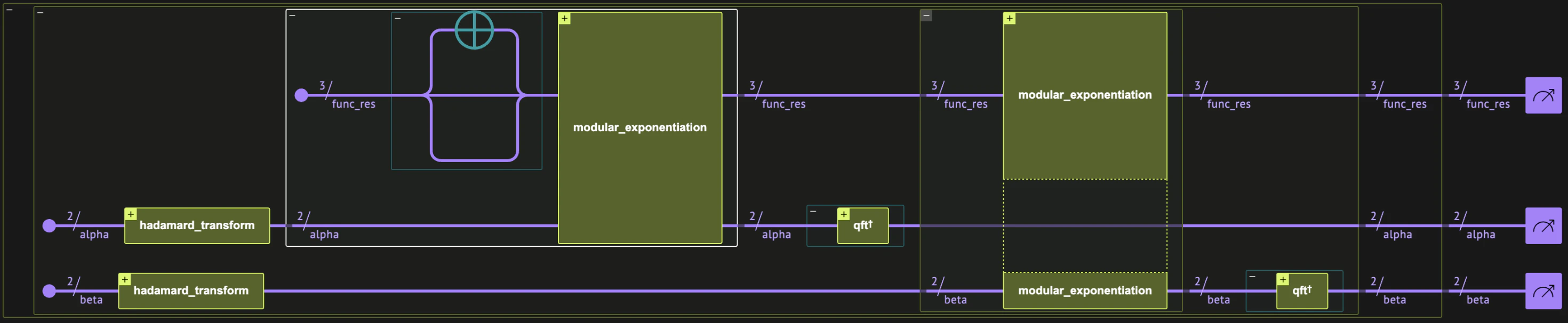
Full Algorithm
- Prepare a uniform superposition over the first two quantum variables
alpha,beta.
- Compute
discrete_log_oracleon thefunc_resvariable.func_resis of size . - Apply the inverse Fourier transform
alpha,beta. - Measure.
func_res variable.
If has an inverse, we can extract from variable by multiplying by .
See the second example for the general case, for which .
Example:
For this specific demonstration, we choose , with and . With this setting, . We choose this specific example because the order of the group is a power of , so we can get the exact discrete logarithm without continued-fractions postprocessing. In other cases, we use a larger quantum variable for the exponents so the continued fractions postprocessing converges.Output:
| alpha | beta | func_res | count | probability | bitstring | |
|---|---|---|---|---|---|---|
| 0 | 2 | 2 | 3 | 268 | 0.06700 | 0111010 |
| 1 | 2 | 2 | 2 | 266 | 0.06650 | 0101010 |
| 2 | 0 | 0 | 3 | 266 | 0.06650 | 0110000 |
| 3 | 0 | 0 | 1 | 264 | 0.06600 | 0010000 |
| 4 | 3 | 1 | 1 | 259 | 0.06475 | 0010111 |
| 5 | 2 | 2 | 1 | 258 | 0.06450 | 0011010 |
| 6 | 1 | 3 | 3 | 256 | 0.06400 | 0111101 |
| 7 | 1 | 3 | 1 | 250 | 0.06250 | 0011101 |
| 8 | 1 | 3 | 4 | 250 | 0.06250 | 1001101 |
| 9 | 3 | 1 | 3 | 246 | 0.06150 | 0110111 |
| 10 | 1 | 3 | 2 | 244 | 0.06100 | 0101101 |
| 11 | 0 | 0 | 4 | 240 | 0.06000 | 1000000 |
| 12 | 3 | 1 | 2 | 238 | 0.05950 | 0100111 |
| 13 | 0 | 0 | 2 | 236 | 0.05900 | 0100000 |
| 14 | 2 | 2 | 4 | 230 | 0.05750 | 1001010 |
| 15 | 3 | 1 | 4 | 229 | 0.05725 | 1000111 |
func_res is uncorrelated to the other variables, and we get uniform distribution, as expected.
We take only the beta that are co-prime to , so they have a multiplicative-inverse.
Hence beta=1,3 are the relevant results.
So we get two relevant results (for all different s): , .
All that remains to get the logarithm is to multiply alpha by the inverse of beta:
Output:
Generalization for the case where
For an arbitrary , we employ two qubit quantum variables and a third -qubit register, initialized to the state , where . The derivation follows a similar structure, where the initial sums are now , with , while the period of remains , i.e., . Therefore, after the second step we obtain the state Next, we express the periodic state in an alternative form. We introduce the operator , which satisfies , where is the identity element of the group. Therefore . The state can be expressed as a uniform superposition of the eigenstates of : where , which satisfy . These relations allow writing the state after the oracle operation as Applying the inverse quantum Fourier transform leads to the state Utilizing the geometric sum, one can show that the functions are peaked (with a width ) around and , correspondingly. To evaluate the values of and we measurealpha and beta registers, multiply by and round.
For sufficiently large , we obtain the correct value for with high probability. Alternatively, one can apply the continued fraction algorithm [5] to evaluate , see [6] for further details.
Note: Alternatively, you could implement the over general , and instead of the uniform superposition, prepare the states: in alpha, beta. Then, again, no continued fractions postprocessing is required.
Example:
Output:
| alpha | beta | func_res | count | probability | bitstring | |
|---|---|---|---|---|---|---|
| 0 | 0.0 | 0.25 | 5 | 91 | 0.0091 | 01010100000000 |
| 1 | 0.0 | 0.25 | 1 | 88 | 0.0088 | 00010100000000 |
| 2 | 0.0 | 0.50 | 10 | 87 | 0.0087 | 10101000000000 |
| 3 | 0.0 | 0.50 | 1 | 85 | 0.0085 | 00011000000000 |
| 4 | 0.0 | 0.50 | 4 | 85 | 0.0085 | 01001000000000 |
| 5 | 0.0 | 0.00 | 4 | 83 | 0.0083 | 01000000000000 |
| 6 | 0.0 | 0.75 | 4 | 83 | 0.0083 | 01001100000000 |
| 7 | 0.0 | 0.50 | 5 | 79 | 0.0079 | 01011000000000 |
| 8 | 0.0 | 0.00 | 12 | 79 | 0.0079 | 11000000000000 |
| 9 | 0.0 | 0.75 | 2 | 78 | 0.0078 | 00101100000000 |
Postprocessing
We now have an additional step in postprocessing. We translate each result to the closest fraction with a denominator, which is the order:| alpha | beta | func_res | count | probability | bitstring | alpha_rounded | beta_rounded | |
|---|---|---|---|---|---|---|---|---|
| 0 | 0.0 | 0.25 | 5 | 91 | 0.0091 | 01010100000000 | 0.0 | 3.0 |
| 1 | 0.0 | 0.25 | 1 | 88 | 0.0088 | 00010100000000 | 0.0 | 3.0 |
| 2 | 0.0 | 0.50 | 10 | 87 | 0.0087 | 10101000000000 | 0.0 | 6.0 |
| 3 | 0.0 | 0.50 | 1 | 85 | 0.0085 | 00011000000000 | 0.0 | 6.0 |
| 4 | 0.0 | 0.50 | 4 | 85 | 0.0085 | 01001000000000 | 0.0 | 6.0 |
| 5 | 0.0 | 0.00 | 4 | 83 | 0.0083 | 01000000000000 | 0.0 | 0.0 |
| 6 | 0.0 | 0.75 | 4 | 83 | 0.0083 | 01001100000000 | 0.0 | 9.0 |
| 7 | 0.0 | 0.50 | 5 | 79 | 0.0079 | 01011000000000 | 0.0 | 6.0 |
| 8 | 0.0 | 0.00 | 12 | 79 | 0.0079 | 11000000000000 | 0.0 | 0.0 |
| 9 | 0.0 | 0.75 | 2 | 78 | 0.0078 | 00101100000000 | 0.0 | 9.0 |
beta is co-prime to the order, such that we can get the logarithm by multiplying alpha by the modular inverse. If the alpha, beta registers are large enough, we are guaranteed to sample it with a good probability:
| alpha | beta | func_res | count | probability | bitstring | alpha_rounded | beta_rounded | beta_inverse | logarithm | |
|---|---|---|---|---|---|---|---|---|---|---|
| 48 | 0.65625 | 0.09375 | 9 | 49 | 0.0049 | 10010001110101 | 8.0 | 1.0 | 1 | 8.0 |
| 50 | 0.34375 | 0.90625 | 1 | 48 | 0.0048 | 00011110101011 | 4.0 | 11.0 | 11 | 8.0 |
| 54 | 0.65625 | 0.09375 | 7 | 42 | 0.0042 | 01110001110101 | 8.0 | 1.0 | 1 | 8.0 |
| 55 | 0.34375 | 0.90625 | 8 | 42 | 0.0042 | 10001110101011 | 4.0 | 11.0 | 11 | 8.0 |
| 58 | 0.65625 | 0.09375 | 10 | 41 | 0.0041 | 10100001110101 | 8.0 | 1.0 | 1 | 8.0 |
| 59 | 0.34375 | 0.90625 | 4 | 40 | 0.0040 | 01001110101011 | 4.0 | 11.0 | 11 | 8.0 |
| 61 | 0.34375 | 0.40625 | 12 | 40 | 0.0040 | 11000110101011 | 4.0 | 5.0 | 5 | 8.0 |
| 66 | 0.65625 | 0.59375 | 2 | 38 | 0.0038 | 00101001110101 | 8.0 | 7.0 | 7 | 8.0 |
| 67 | 0.65625 | 0.59375 | 4 | 38 | 0.0038 | 01001001110101 | 8.0 | 7.0 | 7 | 8.0 |
| 69 | 0.34375 | 0.40625 | 11 | 38 | 0.0038 | 10110110101011 | 4.0 | 5.0 | 5 | 8.0 |
Output:
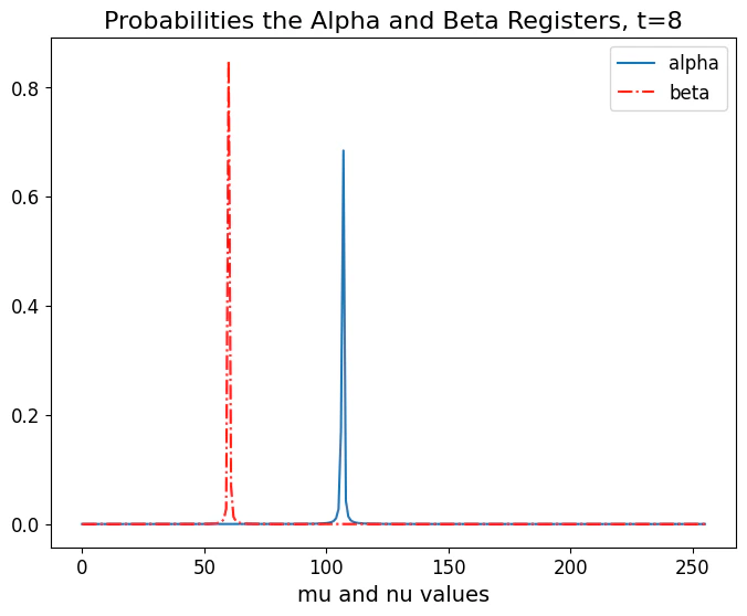
Measurement Distribution Heuristic Plots
The expected measurement results are showcased by plotting the theoretical probability distributions of the and quantum variables, for varying numbers of qubits and and the specific case of . Since for some integer , we obtain a probability distribution characterized by a narrow peak of width . As the number of qubits is increased, increases, the probability distribution becomes narrower. Therefore, improving the success probability.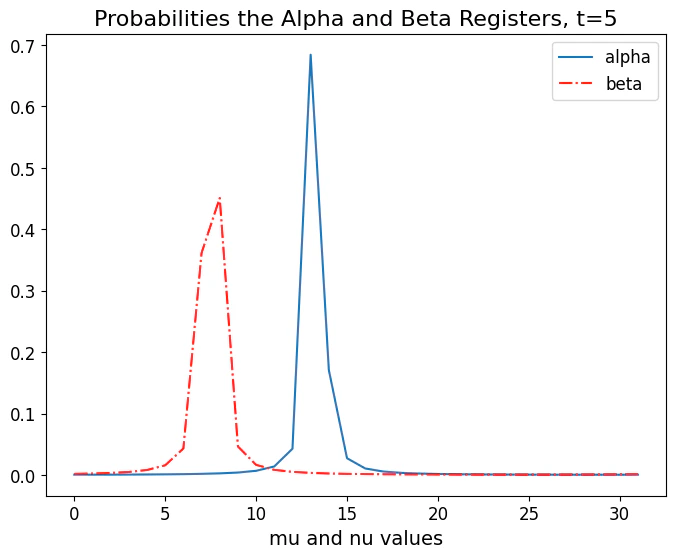
Technical notes
Equivalence with the Abelian subgroup problem
The discrete logarithm is a specific case of the Hidden Subgroup Problem (HSP) [4]. The HSP can be stated as follows: Let be a group and is subgroup of . We are given an (oracle) function with the promise that:- is constant on the right cosets of .
- Elements of distinct cosets produce different oracle values.
- is the additive group .
- The hidden subgroup is .
- The cosets are the of the form , where . It is straightforward to show that for all elements of the coset.
Diffie-Hellman Secret Key Sharing Protocol
The Diffie–Hellman protocol enables two parties (“Alice” and “Bob”) to establish a shared secret key, and its security against an eavesdropper (“Eve”) relies on the computational hardness of the discrete logarithm problem. The protocol for sharing a secret key includes the following steps:- A prime and a generator of a multiplicative group mod , are published publicly.
- Alice chooses a number and computes . is known only to Alice.
- Bob chooses a number and computes . is known only to Bob.
- Alice sends Bob a message over a public channel containing , Bob sends Alice a message containing .
- Alice computes the secret key , and similarly Bob computes the secret key .