Documentation Index
Fetch the complete documentation index at: https://prod-mint.classiq.io/llms.txt
Use this file to discover all available pages before exploring further.
View on GitHub
Open this notebook in GitHub to run it yourself
import numpy as np
import scipy

a_matrix = np.array(
    [
        [0.135, -0.092, -0.011, -0.045, -0.026, -0.033, 0.03, 0.034],
        [-0.092, 0.115, 0.02, 0.017, 0.044, -0.009, -0.015, -0.072],
        [-0.011, 0.02, 0.073, -0.0, -0.068, -0.042, 0.043, -0.011],
        [-0.045, 0.017, -0.0, 0.043, 0.028, 0.027, -0.047, -0.005],
        [-0.026, 0.044, -0.068, 0.028, 0.21, 0.079, -0.177, -0.05],
        [-0.033, -0.009, -0.042, 0.027, 0.079, 0.121, -0.123, 0.021],
        [0.03, -0.015, 0.043, -0.047, -0.177, -0.123, 0.224, 0.011],
        [0.034, -0.072, -0.011, -0.005, -0.05, 0.021, 0.011, 0.076],
    ]
)

b_vector = np.array(
    [
        -0.00885448,
        -0.17725898,
        -0.15441119,
        0.17760157,
        0.41428775,
        0.44735303,
        -0.71137715,
        0.1878808,
    ]
)

sol_classical = np.linalg.solve(a_matrix, b_vector)  # classical solution

# number of qubits for the unitary
num_qubits = int(np.log2(len(b_vector)))
# exact unitary
my_unitary = scipy.linalg.expm(1j * 2 * np.pi * a_matrix)
# transpilation_options = {"classiq": "custom", "qiskit": 3} #uncomment this for deeper comparison
transpilation_options = {"classiq": "auto optimize", "qiskit": 1}
- HHL with Classiq
from classiq import *
from classiq.qmod.symbolic import floor, log


@qfunc
def simple_eig_inv(phase: QNum, indicator: Output[QBit]):
    allocate(indicator)
    assign_amplitude_table(
        lookup_table(lambda p: 0 if p == 0 else (1 / 2**phase.size) / p, phase),
        phase,
        indicator,
    )


@qfunc
def my_hhl(
    precision: int,
    b: CArray[CReal],
    unitary: QCallable[QArray],
    res: Output[QArray],
    phase: Output[QNum],
    indicator: Output[QBit],
) -> None:
    prepare_amplitudes(b, 0.0, res)
    allocate(precision, False, precision, phase)
    within_apply(
        lambda: qpe(unitary=lambda: unitary(res), phase=phase),
        lambda: simple_eig_inv(phase=phase, indicator=indicator),
    )


def get_classiq_hhl_results(precision):
    """
    This function models, synthesizes, executes an HHL example and returns the depth, cx-counts and fidelity
    """

    # SP params
    b_normalized = b_vector.tolist()
    sp_upper = 0.00  # precision of the State Preparation
    unitary_mat = my_unitary.tolist()
    size = (len(b_normalized) - 1).bit_length()

    @qfunc
    def main(res: Output[QNum], phase_var: Output[QNum], indicator: Output[QBit]):
        my_hhl(
            precision=precision,
            b=b_normalized,
            unitary=lambda target: unitary(elements=unitary_mat, target=target),
            res=res,
            phase=phase_var,
            indicator=indicator,
        )

    # Synthesize
    preferences = Preferences(
        custom_hardware_settings=CustomHardwareSettings(basis_gates=["cx", "u"]),
        transpilation_option=transpilation_options["classiq"],
    )
    qprog_hhl = synthesize(main, preferences=preferences)
    total_q = qprog_hhl.data.width  # total number of qubits of the whole circuit
    depth = qprog_hhl.transpiled_circuit.depth
    cx_counts = qprog_hhl.transpiled_circuit.count_ops["cx"]

    # Execute
    backend_preferences = ClassiqBackendPreferences(
        backend_name=ClassiqSimulatorBackendNames.SIMULATOR_STATEVECTOR
    )
    execution_preferences = ExecutionPreferences(
        num_shots=1, backend_preferences=backend_preferences
    )

    with ExecutionSession(qprog_hhl, execution_preferences) as es:
        result = es.sample()

    df = result.dataframe
    qsol = np.zeros(2**size, dtype=complex)

    # Post-process
    # Filter only the successful states.
    filtered_st = df[
        (df.indicator == 1) & (df.phase_var == 0) & (np.abs(df.amplitude) > 1e-12)
    ]

    # Allocate values
    qsol[filtered_st.res] = filtered_st.amplitude / (1 / 2**precision)

    fidelity = (
        np.abs(
            np.dot(
                sol_classical / np.linalg.norm(sol_classical),
                qsol / np.linalg.norm(qsol),
            )
        )
        ** 2
    )
    return total_q, depth, cx_counts, fidelity
classiq_widths = []
classiq_depths = []
classiq_cx_counts = []
classiq_fidelities = []
for per in range(2, 9):
    total_q, depth, cx_counts, fidelity = get_classiq_hhl_results(per)
    classiq_widths.append(total_q)
    classiq_depths.append(depth)
    classiq_cx_counts.append(cx_counts)
    classiq_fidelities.append(fidelity)
print("classiq overlap:", classiq_fidelities)
print("classiq depth:", classiq_depths)
Output:
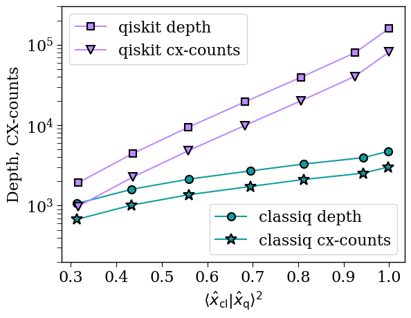
classiq overlap: [0.31375840880338923, 0.4338789033788851, 0.5603091264685023, 0.6943614908054292, 0.8120393433685461, 0.9428405526765191, 0.9982198481096445]
  classiq depth: [1063, 1598, 2141, 2700, 3291, 3946, 4729]
- Comparing to Qiskit
- To run the qiskit code uncomment the commented cells below.
qiskit_fidelities = [
    0.3158037121175521,
    0.43599529278857063,
    0.5586003448231571,
    0.6824252904259536,
    0.806169290650212,
    0.9243747525650154,
    1.0,
]
qiskit_depths = [1921, 4439, 9451, 19455, 39443, 79399, 159291]
qiskit_widths = [6, 7, 8, 9, 10, 11, 12]
qiskit_cx_counts = [979, 2263, 4819, 9915, 20087, 40407, 81019]
# from importlib.metadata import version
# try:
#     import qiskit
#     if version('qiskit') != "1.0.0":
#       !pip uninstall qiskit -y
#       !pip install qiskit==1.0.0
# except ImportError:
#     !pip install qiskit==1.0.0
# from qiskit import QuantumCircuit, QuantumRegister, transpile
# from qiskit.quantum_info import Statevector
# from qiskit.circuit.library import PhaseEstimation as PhaseEstimation_QISKIT
# from qiskit.circuit.library.arithmetic.exact_reciprocal import ExactReciprocal
# from qiskit.circuit.library import Isometry, Initialize

# def get_qiskit_hhl_results(precision):
#     """
#     This function creates an HHL circuit with qiskit, execute it and returns the depth, cx-counts and fidelity
#     """

#     vector_circuit = QuantumCircuit(num_qubits)
#     initi_vec = Initialize(b_vector / np.linalg.norm(b_vector))

#     vector_circuit.append(
#         initi_vec, list(range(num_qubits))
#     )

#     q = QuantumRegister(num_qubits, "q")
#     unitary_qc = QuantumCircuit(q)
#     unitary_qc.unitary(my_unitary.tolist(), q)
#     qpe_qc = PhaseEstimation_QISKIT(precision, unitary_qc)
#     reciprocal_circuit = ExactReciprocal(
#         num_state_qubits=precision, scaling=1 / 2**precision
#     )
#     # Initialise the quantum registers
#     qb = QuantumRegister(num_qubits)  # right hand side and solution
#     ql = QuantumRegister(precision)  # eigenvalue evaluation qubits
#     qf = QuantumRegister(1)  # flag qubits

#     hhl_qc = QuantumCircuit(qb, ql, qf)

#     # State preparation
#     hhl_qc.append(vector_circuit, qb[:])
#     # QPE
#     hhl_qc.append(qpe_qc, ql[:] + qb[:])
#     # Conditioned rotation
#     hhl_qc.append(reciprocal_circuit, ql[::-1] + [qf[0]])

#     # QPE inverse
#     hhl_qc.append(qpe_qc.inverse(), ql[:] + qb[:])

#     # transpile
#     tqc = transpile(
#         hhl_qc,
#         basis_gates=["u3", "cx"],
#         optimization_level=transpilation_options["qiskit"],
#     )
#     depth = tqc.depth()
#     cx_counts = tqc.count_ops()["cx"]
#     total_q = tqc.width()

#     # execute
#     statevector = np.array(Statevector(tqc))

#     # post_process
#     all_entries = [np.binary_repr(k, total_q) for k in range(2**total_q)]
#     sol_indices = [
#         int(entry, 2)
#         for entry in all_entries
#         if entry[0] == "1" and entry[1 : precision + 1] == "0" * precision
#     ]
#     qsol = statevector[sol_indices] / (1 / 2**precision)

#     sol_classical = np.linalg.solve(a_matrix, b_vector)
#     fidelity = (
#         np.abs(
#             np.dot(
#                 sol_classical / np.linalg.norm(sol_classical),
#                 qsol / np.linalg.norm(qsol),
#             )
#         )
#         ** 2
#     )

#     return total_q, depth, cx_counts, fidelity
# qiskit_widths = []
# qiskit_depths = []
# qiskit_cx_counts = []
# qiskit_fidelities = []

# for per in range(2, 9):
#     total_q, depth, cx_counts, fidelity = get_qiskit_hhl_results(per)
#     qiskit_widths.append(total_q)
#     qiskit_depths.append(depth)
#     qiskit_cx_counts.append(cx_counts)
#     qiskit_fidelities.append(fidelity)
- Plotting the Data
import matplotlib.pyplot as plt

classiq_color = "#119DA4"
qiskit_color = "#bb8bff"
plt.rcParams["font.family"] = "serif"
plt.rc("savefig", dpi=300)

plt.rcParams["axes.linewidth"] = 1
plt.rcParams["xtick.major.size"] = 5
plt.rcParams["xtick.minor.size"] = 5
plt.rcParams["ytick.major.size"] = 5
plt.rcParams["ytick.minor.size"] = 5


(classiq1,) = plt.semilogy(
    classiq_fidelities,
    classiq_depths,
    "-o",
    label="classiq depth",
    markerfacecolor=classiq_color,
    markeredgecolor="k",
    markersize=8,
    markeredgewidth=1.5,
    linewidth=1.5,
    color=classiq_color,
)
(classiq2,) = plt.semilogy(
    classiq_fidelities,
    classiq_cx_counts,
    "-*",
    label="classiq cx-counts",
    markerfacecolor=classiq_color,
    markeredgecolor="k",
    markersize=12,
    markeredgewidth=1.5,
    linewidth=1.5,
    color=classiq_color,
)
(qiskit1,) = plt.semilogy(
    qiskit_fidelities,
    qiskit_depths,
    "-s",
    label="qiskit depth",
    markerfacecolor=qiskit_color,
    markeredgecolor="k",
    markersize=7,
    markeredgewidth=1.5,
    linewidth=1.5,
    color=qiskit_color,
)
(qiskit2,) = plt.semilogy(
    qiskit_fidelities,
    qiskit_cx_counts,
    "-v",
    label="qiskit cx-counts",
    markerfacecolor=qiskit_color,
    markeredgecolor="k",
    markersize=8,
    markeredgewidth=1.5,
    linewidth=1.5,
    color=qiskit_color,
)

first_legend = plt.legend(
    handles=[qiskit1, qiskit2],
    fontsize=16,
    loc="upper left",
)
ax = plt.gca().add_artist(first_legend)
plt.legend(handles=[classiq1, classiq2], fontsize=16, loc="lower right")

# plt.ylim(0.2e3,2e5)
plt.ylim(0.2e3, 3e5)
plt.ylabel("Depth, CX-counts", fontsize=16)
plt.xlabel(r"$\langle\hat{x}_{\rm cl}|\hat{x}_{\rm q}\rangle^2$", fontsize=16)
plt.yticks(fontsize=16)
plt.xticks(fontsize=16)
Output:
(array([0.2, 0.3, 0.4, 0.5, 0.6, 0.7, 0.8, 0.9,

1. , 1.1]),
   [Text(0.2, 0, '0.2'),
    Text(0.30000000000000004, 0, '0.3'),
    Text(0.4, 0, '0.4'),
    Text(0.5, 0, '0.5'),
    Text(0.6000000000000001, 0, '0.6'),
    Text(0.7, 0, '0.7'),
    Text(0.8, 0, '0.8'),
    Text(0.9000000000000001, 0, '0.9'),
    Text(1.0, 0, '1.0'),
    Text(1.1, 0, '1.1')])