Bernstein-Vazirani Algorithm
The Bernstein-Vazirani (BV) algorithm [1], named after Ethan Bernstein and Umesh Vazirani, is a fundamental quantum algorithm that demonstrates a linear speed-up compared to its classical counterpart in the oracle complexity setting. While the BV algorithm showcases this theoretical speed-up, its practical utility is limited due to its specific problem domain. Nonetheless, it stands as one of the early examples illustrating the potential of quantum computing to outperform classical methods in certain scenarios.
The algorithm addresses the following problem:
-
Given an $ n $-bit string $ x $ representing the input of a function $ f:{0,1}^n \rightarrow {0,1} $.
-
$ f $ is a "quantum oracle function" (see NOTE) that takes an $ n $-bit string as input and returns the inner product of the input string and the "hidden bit string" $ s $: $ f(x) = x \cdot s $ for all $ x $, where the inner product is computed modulo 2.
Summing-up:
Input: $ x $, an $ n $-bit string.
Promise: There exists a hidden $ n $-bit string $ s $ such that $ f(x) = x \cdot s $ for all $ x $.
The goal: Determine the hidden bit string $ s $ using the minimal number of queries (evaluations) of the oracle function $ f $.
NOTE regarding the oracle function:
For the sake of this tutorial you could think of oracle function as "black-box" function, but we include here little elaboration: The standard way [[2](#NielsenChuang)] to apply a classical function $f:\{0,1\}^n \rightarrow \{0,1\}$ on quantum states is with the oracle model: $\begin{equation} O_f (\ket{x}_n\ket{y}_1) = \ket{x}_n\ket{y \oplus f(x)}_1 \end{equation}$ with $\ket{x}$ and $\ket{y}$ being the argument and target quantum states respectively, and $\oplus$ being addition modolu $2$, or the XOR operation. The BV algorithm takes the oracle $O_f$ as an input, and performs the following operation: $\begin{equation} \ket{x}\rightarrow (-1)^{f(x)}\ket{x}. \end{equation}$ This can be applied on a superposition of states such that $\begin{equation} \sum_{i=0}^{2^n-1}\alpha_i\ket{x_i}\rightarrow (-1)^{f(x_i)}\alpha_i\ket{x_i} \end{equation}$ with $\alpha_i$ being the amplitude of the $\ket{x_i}$ state. How does this happen? It is simple (hence the beauty of it). Apply the oracle $O_f$ to the state target quantum state $\ket{-}=\frac{1}{\sqrt{2}}\ket{0}-\frac{1}{\sqrt{2}}\ket{1}$ such that $\begin{equation} O_f\ket{x}\ket{-} = (-1)^{f(x)}\ket{x}\ket{-} \end{equation}$ and then effectively achieving the desired transformation $\ket{x}\rightarrow (-1)^{f(x)}\ket{x}$.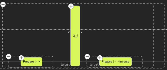
The best classical solution for this problem typically requires $ n $ evaluations of the function $ f $ to determine the hidden bit string $ s $. This scenario arises when the input bit string $ x $ consists of $ n-1 $ zeros and a single one, which systematically shifts across all positions in the string to explore all possible linear combinations.
For example, the first evaluation would set $ x = 100...0 $, the second evaluation $ x = 010...0 $, and so on.
In contrast to the classical solution, the quantum solution requires only a single query.
See how this works in the Mathematical Description.
Classiq Concepts * [Within-apply](https://docs.classiq.io/latest/qmod-reference/language-reference/statements/within-apply/ * Classical Control Flow (repeat, if_)
Guided Implementation
The quantum solution that exploits this advantage takes the following steps:
1. Prepare a uniform superposition in the input state $ x $ using hadamard_transform.
2. Apply the oracle function that implements the function $ f $ Within $ \ket{-} $.
3. Reapply uniform superposition on the registers of $ x $.
The first and last steps could be easily done in the main function using the Classiq built-in hadamard_transform(). The second step is more complex. Break it down, bearing in mind that with Classiq--as with any serious development platform--it is recommended to design your code at the functional level in terms of functions.
According to this note, implement one function at a time and then connect them.
Let's start implementing!
The main building block in the implementation uses within_apply. This Classiq function performs the common quantum pattern: $ U^{\dagger}VU \(.
This function contains two nested statement blocks--the compute block and the action block--and evaluates this sequence: compute (\) U \(), action (\) V \(), and invert(compute) (\) U^{\dagger} $).
According to the algorithm, $ U $ is chosen to be prepare_minus on the auxiliary qubit, while $ V $ is the unitary oracle operator ($ O_f $) that implements the function $ f $.
Use the prepare \(\ket{-}\) building block implemented with the prepare_minus function. Implement it by sequentially applying the X (NOT) gate that transforms \(\ket{0}\) into \(X\ket{0}=\ket{1}\), and then applying the Hadamard H gate that takes the \(\ket{1}\) state into the desired \(H\ket{1}=\ket{-}\) state:
from classiq import H, Output, QBit, X, allocate, qfunc


@qfunc
def prepare_minus(target: Output[QBit]):
    allocate(out=target, num_qubits=1)
    X(target)
    H(target)
Apply the oracle operator ($ O_f $) that implements the function $ f $.
It is possible to implement $ O_f $ using an auxiliary qubit that registers the value of $ f(x) $ by following this logic:
* For each \(s_i =1\), apply $ X $ gate on the auxiliary $ \ket{f} $ controlled by $ \ket{x_i} $.
* If $ s_i=0 $, do nothing, which is equivalent to applying the IDENTITY function.
from classiq import CX, IDENTITY, CInt, QArray, if_, repeat
from classiq.qmod.symbolic import floor


@qfunc
def oracle_function(s: CInt, x: QArray, res: QBit):

    repeat(
        count=x.len,
        iteration=lambda i: if_(
            condition=floor(s / 2**i) % 2 == 1,
            then=lambda: CX(x[i], res),
            else_=lambda: IDENTITY(res),
        ),
    )
- Here, the "oracle_function" employs the
repeatconstruct to execute the logic described earlier $ n $ times (length of $ x $), as specified by the parameter 'count'. - Each iteration of the
repeatloop utilizes theif_statement, which parallels the conventional Python 'if' statement. It comprises the 'condition', 'then', and 'else_' attributes, which mirror the structure of an if-else statement in native Python.
Loops and conditions are the bread and butter of classical computation. Qmod, the Classiq native language accessed through the Classiq Python SDK, employs the same concepts with repeat and if_ statements, serving as a means of Classical Control Flow. These are handy tools for describing reusable building blocks.
The 'condition' looks confusing at a first glance, but all it does is implement the above mentioned logic examining the value of $ s_i \in {0,1}$ to apply the appropriate gate.
Breaking it down:
-
$ \text{floor}(s / 2^i) $ divides the secret integer $ s $ by $ 2^i $, effectively shifting the bits of $ s $, $ i $ positions to the right in the binary representation.
-
Taking the result modulo 2 then extracts the most significant bit of the resulting number.
-
If the extracted bit is 1, it indicates that the $ i $-th bit of the binary representation of $ s $ is indeed 1.
In summary:
-
The
conditionin theif_statement checks whether the bit value at position \(i\) is 1 or 0. -
If the condition is true (i.e., the bit value is 1), the
thenblock applies a controlled-NOT (CX) gate. -
If the condition is false (i.e., the bit value is 0), the
else_block does nothing and uses theIDENTITYgate.
You are almost done. \
Now you have all you need to set the 'bv_function' using within_apply, as discussed earlier:
from classiq import within_apply


@qfunc
def bv_function(s: CInt, x: QArray[QBit]):

    aux = QBit("aux")
    within_apply(lambda: prepare_minus(aux), lambda: oracle_function(s, x, aux))
Begin by initializing an auxiliary qubit called "aux". Then, leverage within_apply (learn more here as discussed previously: $ U=$ prepare_minus(aux) and $ V=$f_logic(s, x, aux).
You receive the desired logic:
Finally, assemble all your building blocks in the main function:
from classiq import QNum, hadamard_transform


@qfunc
def main(x: Output[QNum]):

    allocate(STRING_LENGTH, x)

    hadamard_transform(x)
    bv_function(SECRET_INT, x)
    hadamard_transform(x)
Let's check what you have created!
# Input values:
SECRET_INT = 13  # We expect to get it as output
STRING_LENGTH = 5
NUM_SHOTS = 1
Note that the number of shots can be set to 1, under the assumption of noiseless execution.
# Make sure the input makes sense:
import numpy as np

assert (
    np.floor(np.log2(SECRET_INT) + 1) <= STRING_LENGTH
), "The STRING_LENGTH cannot be smaller than the secret string length"
Execution:
from classiq import create_model, execute, set_execution_preferences, show, synthesize
from classiq.execution import ExecutionPreferences

# Creating the model using `ExecutionPreferences` of the desired number of shots:
execution_preferences = ExecutionPreferences(num_shots=NUM_SHOTS)
# qmod = set_execution_preferences(qmod, execution_preferences)
qmod = create_model(
    main, execution_preferences=ExecutionPreferences(num_shots=NUM_SHOTS)
)

# Synthesizing the optimized circuit (quantum program) of the model in the Classiq backend:
qprog = synthesize(qmod)

# Showing the quantum program using the Classiq visualizer
show(qprog)
Before executing the program and making sure it actually works, play with the Classiq super cool visualization tool! It is very convenient to see the different building blocks and hierarchies in the program.

Verify that the quantum program actually does what you expect.
Execution with one shot yields this:
# Execute the quantum program and access the result
job = execute(qprog)
res = execute(qprog).result()
secret_integer_q = res[0].value.parsed_counts[0].state["x"]

print("The secret integer is:", secret_integer_q)
print(
    "The probability for measuring the secret integer is:",
    res[0].value.parsed_counts[0].shots / NUM_SHOTS,
)
The secret integer is: 13.0
The probability for measuring the secret integer is: 1.0
You received the expected result!
Using only one approximation of the function, you demonstrated the hidden power in quantum computation. \
As mentioned before, the best classical calculation would have taken STRING_LENGTH approximations on a classical computer.
You could also execute using the platform GUI. After setting the number of shots and executing, you would receive this:

Or if you want to explore the execution after running it from the notebook:
job.open_in_ide()
Mathematical Description
Here's the Bernstein-Vazirani algorithm described mathematically:
The starting point by definition is the $ n $ dimensional zero state:
The first step in the algorithm is to apply a Hadamard gate to each qubit:
when $ \ket{x} $ is the integer basis in binary representation.
Then, apply the oracle $ O_f $ by definition:
The state \(\ket{-}\) is the state of the auxiliary qubit in our code. The value of \(f(x)\), \(1\) or \(0\) determine whether there is phase flip or not correspondingly.
You actually apply the oracle on the state \(\ket{X}\) and not on the superposition component \(\ket{x}\), so you get this state:
Now after applying the oracle, we apply Hadamard gates again to each qubit except the auxiliary qubit which could be left aside:
We obtain $ \ket{s} $ because for each $ \ket{y} $, the coefficient is equal to 1 only if $ s \oplus y = \vec{0} $. Otherwise, the coefficient is 0.
Note that $ s \oplus y = \vec{0} $ occurs only when $ s = y $, meaning only one component contributes to the sum. This component is $ \ket{y} = \ket{s} $ with a coefficient of 1.
All Code Together
Python version:
from classiq import *
from classiq.execution import ExecutionPreferences
from classiq.qmod.symbolic import floor


@qfunc
def prepare_minus(target: Output[QBit]):
    allocate(out=target, num_qubits=1)
    X(target)
    H(target)


@qfunc
def bv_predicate(a: CInt, x: QArray, res: QBit):

    repeat(
        x.len,
        lambda i: if_(
            floor(a / 2**i) % 2 == 1, lambda: CX(x[i], res), lambda: IDENTITY(res)
        ),
    )


@qfunc
def bv_function(a: CInt, x: QArray):

    aux = QBit("aux")
    within_apply(lambda: prepare_minus(aux), lambda: bv_predicate(a, x, aux))


SECRET_INT = 13
STRING_LENGTH = 5
NUM_SHOTS = 1  # Could be set to 1 under the assumption of noiseless execution


@qfunc
def main(x: Output[QNum]):
    allocate(STRING_LENGTH, x)
    hadamard_transform(x)
    bv_function(SECRET_INT, x)
    hadamard_transform(x)


qmod = create_model(
    main, execution_preferences=ExecutionPreferences(num_shots=NUM_SHOTS)
)
qprog = synthesize(qmod)
write_qmod(qmod, "bv_tutorial")
job = execute(qprog)
job.open_in_ide()

# show(qprog) # uncomment to review the circuit
References
[1]: Bernstein–Vazirani algorithm (Wikipedia)
[2]: Quantum Computation and Quantum Information (Michael Nielsen and Isaac Chuang)