Classiq Overview Tutorial

In this notebook we introduce a typical workflow with Classiq:

Designing a quantum model using the Qmod language and it's accompanied function library.
Synthesizing the model into a concrete circuit implementation.
Executing the program on a chosen simulator or quantum hardware.
Post-processing the results.

Later tutorials dive into each of the above stages, providing hands-on interactive guides that go from the very basics to advanced usage.

To get started, run:

from classiq import *

If this import doesn't work for you, please try pip install classiq in your terminal, or refer to Registration and Installation.

Designing a Quantum Model

Here we will define a quantum function main that calculates a simple arithmetic expression:

@qfunc
def main(x: Output[QNum], y: Output[QNum]) -> None:
    allocate(3,x)
    hadamard_transform(x)
    y |= x**2 + 1

Explaining the code step-by-step:

Allocate 3 qbits for the quantum number x, so that it can represent \(2^3\) different numbers, from 0 to 7 (for example, the bitstring '010' represents the number 2).
Apply hadamard_transform to x, creating an equal superposition of all these values.
Assign the desired arithmetic expression's result to the quantum number y.

A moment before measurement, we expect the output variables x and y to be in an equal superposition of the states \(|x_i\rangle |y_i=x_i^2+1\rangle\) for \(x_is\) from 0 to 7. In other words, we have designed our quantum model to calculate \(x^2 +1\).

Synthesizing The Model

The function main describes the model in a high-level manner: "calculate \(x^2+1\) and assign in into y". However, it does not specify how to implement this calculation - it does not map it to an executable quantum circuit, in terms of elementary quantum gates applied to specific qubits. In order to do so, we use Classiq's synthesis engine.

First, create a Quantum Model object qmod out of the function main:

qmod = create_model(main)

Then, pass qmod to the synthesis engine to obtain a concrete quantum program qprog. Here we simply call the function synthesize. Later on we will learn to provide configuration details (e.g. which elementary gates are allowed, or what resources we are trying to optimize).

qprog = synthesize(qmod)

We can analyze the resulting implementation using Classiq's visualization tool:

show(qprog)

Opening: https://platform.classiq.io/circuit/2sdF7ey6Azju9VOkicpb93WuI8Y?version=0.67.0

This should pop up a web page with something like this:

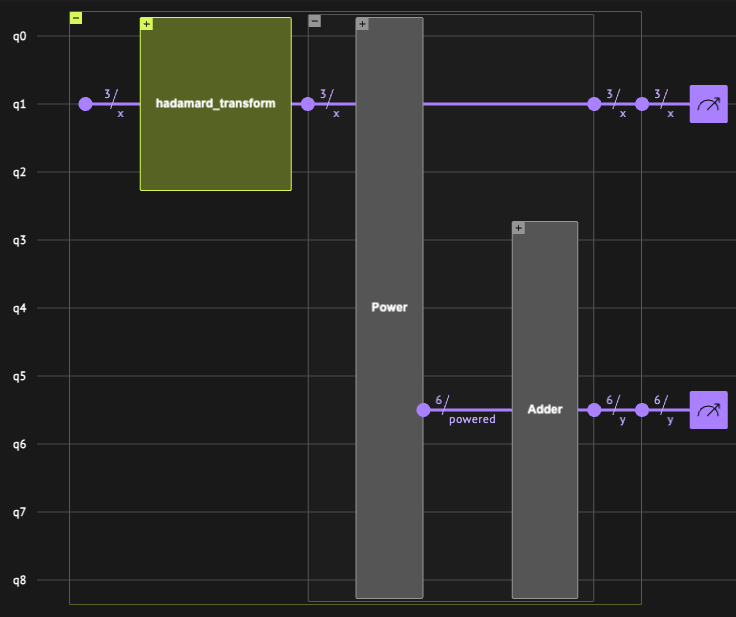
By clicking the + icons on the blocks' top-left corner, we can inspect the gate-level implementation of each functional block. For example, inspect the complex combination of H, CPHASE, CX and U gates that implements the Power block.

Executing The Quantum Program

Now that we have a concrete circuit implementation of the desired model, we can execute it and sample the resulting states of the output variables. Here we will simply call the function execute, which uses Classiq's default quantum simulator and samples the variable multiple times (the default n_shots is 2048):

job = execute(qprog)

Later on we will learn how to execute on hardwares and simulators of our choice and manage advanced executions (for example, hybrid execution that uses classical logic to alter the circuit between runs).

Post-processing The Results

Having executed the quantum program multiple times (n_shots=2048) we can now inspect the possible pairs x,y that our arithmetic expression allows (\(y=x^2+1\)). This can be done by looking into parsed_counts - a list of all the states that were measured on the output variables, ordered by the number of shots (counts) that they were measured.

pc = job.get_sample_result().parsed_counts
print(pc)

[{'x': 6, 'y': 37}: 280, {'x': 1, 'y': 2}: 278, {'x': 0, 'y': 1}: 272, {'x': 7, 'y': 50}: 253, {'x': 3, 'y': 10}: 252, {'x': 5, 'y': 26}: 244, {'x': 4, 'y': 17}: 239, {'x': 2, 'y': 5}: 230]

As expected, all possible values of x (integers from 0 to 7) were measured roughly similar number of times, and with each x measured, the measurement of y satisfies \(y=x^2+1\).

Alternatively, you can inspect the histogram of sampled states in Classiq's web platform:

job.open_in_ide()

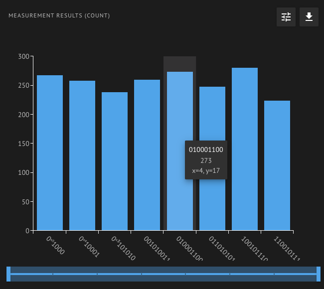
Hovering above each of the histogram bars shows its bitstring and its parsed variables values. For example, the bitstring '010001100' is parsed as x=4, y=17, because the first 3 qubits (counting from the right) correspond to x and were measured as '100'=4 (in binary), and the other 6 qubits which correspond to y were measured as '010001'=17.

Summary

In this tutorial, we have gone through a typical workflow using Classiq:

Designing a quantum model: the problem we wanted to solve is calculating an arithmetic expression for a given domain of x values. We used hadamard_transform and arithmetic assignment as our modeling building blocks.
Synthesizing the model into a concrete circuit implementation: we called synthesize to let Classiq's synthesis engine take our high-level description and implement it in an executable way.
Executing the program: we called execute to run our quantum program multiple times on Classiq's simulator.
Post-processing: We inspected the measured states of x and y - for each x and assured ourselves that they satisfy the desired arithmetic expression.

Food for Thought

You might have noticed that the model discussed here does not truly harness the power of quantum computers: a moment before sampling the qubits, x and y indeed hold "the answers to all questions" simultaneously (all the pairs x and y that satisfy the equation), but we cannot access these answers until we measure the qubits, which collapses the superposition and leaves only a single (and randomly chosen) pair of x and y.

Having said that, we have no choice but to run multiple times (many more than \(2^3\) in our case) to make sure that we measure all xs of interest. A classical computer could obtain the same information in exactly \(2^3\) runs.

Then, why bother?

While pure arithmetic alone may never be a primary task for quantum computers, quantum arithmetic plays a crucial role in many quantum algorithms that do exploit quantum speedup. For example, it is widely used in oracle functions within Grover’s search algorithm and in quantum cryptographic protocols.

Practice

Edit the arithmetic expression inside main, using the +, -, ** operators as well as literal numbers of your choice. Validate that the sampled states of x and y satsify your arithmetic expression.