View on GitHub
Open this notebook in GitHub to run it yourself
Introduction
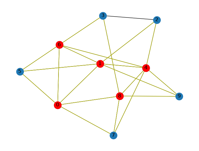
The Max K-Vertex Cover problem [1] is a classical problem in graph theory and computer science, where we aim to find a set of vertices such that each edge of the graph is incident to at least one vertex in the set, and the size of the set does not exceed a given number .Mathematical Formulation
The Max-k Vertex Cover problem can be formulated as an Integer Linear Program (ILP): Minimize: Subject to: and Where:- is a binary variable that equals 1 if node is in the cover and 0 otherwise
- is the set of edges in the graph
- is the set of vertices in the graph
- is the maximum number of vertices allowed in the cover
Solving with the Classiq Platform
We go through the steps of solving the problem with the Classiq platform, using QAOA algorithm [2]. The solution is based on defining a Pyomo model for the optimization problem we would like to solve.Building the Pyomo Model from a Graph Input
We proceed by defining the Pyomo model that will be used on the Classiq platform, using the mathematical formulation defined above:- Index set declarations (model.Nodes, model.Arcs).
- Binary variable declaration for each node (model.x) indicating whether the variable is chosen for the set.
- Constraint rule - ensures that the set is of size k.
- Objective rule - counts the number of edges not covered; i.e., both related variables are zero.
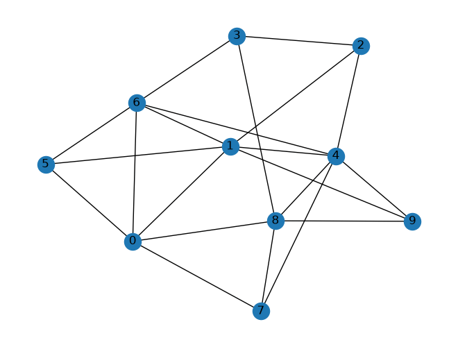
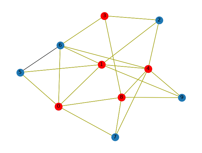
Output:
Setting Up the Classiq Problem Instance
In order to solve the Pyomo model defined above, we use theCombinatorialProblem python class.
Under the hood it tranlates the Pyomo model to a quantum model of the QAOA algorithm, with cost hamiltonian translated from the Pyomo model. We can choose the number of layers for the QAOA ansatz using the argument num_layers, and the penalty_factor, which will be the coefficient of the constraints term in the cost hamiltonian.
Synthesizing the QAOA Circuit and Solving the Problem
We can now synthesize and view the QAOA circuit (ansatz) used to solve the optimization problem:Output:
Output:
optimize method of the CombinatorialProblem object.
For the classical optimization part of the QAOA algorithm we define the maximum number of classical iterations (maxiter) and the -parameter (quantile) for running CVaR-QAOA, an improved variation of the QAOA algorithm [3]:
Output:
Output:
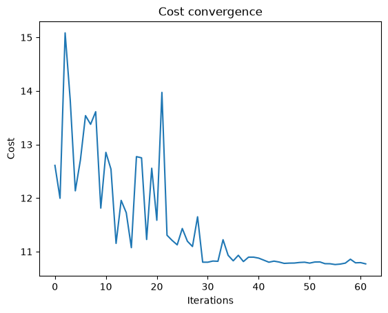
Optimization Results
We can also examine the statistics of the algorithm. In order to get samples with the optimized parameters, we call thesample method:
We will also want to compare the optimized results to uniformly sampled results:
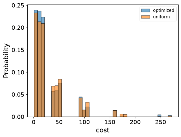
Output:
Comparison to a Classical Solver
Lastly, we can compare to the classical solution of the problem:Output: