> ## Documentation Index
> Fetch the complete documentation index at: https://docs.classiq.io/llms.txt
> Use this file to discover all available pages before exploring further.
# Quantum linear solver with LCU of Chebyshev polynomials
Open this notebook in GitHub to run it yourself
The code here can be integrated as part of a larger CFD solver, e.g., as in [qc-cfd repository](https://github.com/rolls-royce/qc-cfd/tree/main/1D-Nozzle).
In particular, instead of calling a classical solver, e.g., `x = sparse.linalg.spsolve(mat_raw_scr, b_raw)`, one can call the quantum solver `cheb_lcu_approx_solver(mat_raw_scr, b_raw,...)`.
We implemented two versions for block-encoding, one based on Pauli decomposition of the matrix, and another one based on decomposing the matrix to a finite set of diagonals.
```python theme={null}
!pip install -qq "classiq[qsp]"
!pip install -qq "classiq[chemistry]"
```
We start with defining the functions.
First we define the quantum function `lcu_cheb_approx` that implements an approximated Chebyshev LCU quantum linear solver.
```python theme={null}
import time
import matplotlib.pyplot as plt
import numpy as np
from banded_be import get_banded_diags_be
from cheb_utils import *
from classical_functions_be import get_svd_range
from pauli_be import get_pauli_be
from scipy import sparse
from classiq import *
from classiq.applications.qsp.qsp import poly_inversion
np.random.seed(53)
PAULI_TRIM_REL_TOL = 0.1
```
```python theme={null}
from classiq.qmod.symbolic import pi
@qfunc
def my_reflect_about_zero(qba: QNum):
reflect_about_zero(qba)
phase(pi)
@qfunc
def walk_operator(
block_enc: QCallable[QArray, QArray], block: QArray, data: QArray
) -> None:
block_enc(block, data)
my_reflect_about_zero(block)
@qfunc
def symmetrize_walk_operator(
block_enc: QCallable[QNum, QArray], block: QNum, data: QArray
):
my_reflect_about_zero(block)
within_apply(
lambda: block_enc(block, data),
lambda: my_reflect_about_zero(block),
)
@qfunc
def lcu_cheb_approx(
powers: CArray[CInt],
inv_coeffs: CArray[CReal],
sp_error: CReal,
block_enc: QCallable[QNum, QArray],
mat_block: QNum,
data: QArray,
cheb_block: QArray,
) -> None:
within_apply(
lambda: inplace_prepare_state(inv_coeffs, sp_error, cheb_block),
lambda: (
Z(cheb_block[0]),
repeat(
powers.len,
lambda i: control(
cheb_block[i],
lambda: power(
powers[i],
lambda: symmetrize_walk_operator(block_enc, mat_block, data),
),
),
),
my_reflect_about_zero(mat_block),
walk_operator(block_enc, mat_block, data),
),
)
```
Next, we define the `cheb_lcu_approx_solver` function, which gets the matrix and right-hand-side vector, applies the quantum solver, and returns the linear equation solution using a statevector simulator.
The solvers in this directory were developed in the framework of exploring their performance in hybrid CFD schemes.
For simplicity, it is assumed that all the properties of the matrices are known explicitly. In particular, we calculate its singular values for identifying the range in which we apply the inversion polynomial.
```python theme={null}
def cheb_lcu_approx_solver(
mat_raw_scr,
b_raw,
log_poly_degree,
be_method="banded",
approximation=0,
preferences=Preferences(),
constraints=Constraints(),
):
scale = 0.5
b_norm = np.linalg.norm(b_raw)
b_normalized = b_raw / b_norm
data_size = max(1, (len(b_raw) - 1).bit_length())
if be_method == "pauli":
data_size, block_size, be_scaling_factor, be_qfunc = get_pauli_be(mat_raw_scr)
if be_method == "banded":
data_size, block_size, be_scaling_factor, be_qfunc = get_banded_diags_be(
mat_raw_scr
)
w_min, w_max = get_svd_range(mat_raw_scr / be_scaling_factor)
poly_degree = 2 * (2**log_poly_degree - 1) + 1
c, m = poly_inversion(poly_degree, 1 / w_min, "relative")
pcoefs, poly_scale = scale * c / m, scale / m
odd_coef = pcoefs[1::2]
if approximation > 0:
odd_coef = fit_linear_coeffs_for_cheb(pcoefs)
lcu_size_inv = len(odd_coef).bit_length() - 1
print(f"Chebyshev LCU size: {lcu_size_inv} qubits.")
odd_coeffs_signs = np.sign(odd_coef)
assert np.all(
odd_coeffs_signs == np.where(np.arange(len(odd_coeffs_signs)) % 2 == 0, 1, -1)
), "Non alternating signs for odd coefficients"
normalization_inv = sum(np.abs(odd_coef))
print(f"Normalization factor for inversion: {normalization_inv}")
prepare_probs_inv = (np.abs(odd_coef) / normalization_inv).tolist()
@qfunc
def main(
matrix_block: Output[QNum[block_size]],
data: Output[QNum[data_size]],
inv_block: Output[QNum[lcu_size_inv]],
):
allocate(inv_block)
allocate(matrix_block)
prepare_amplitudes(b_normalized.tolist(), 0, data)
lcu_cheb_approx(
powers=[2**i for i in range(lcu_size_inv)],
inv_coeffs=prepare_probs_inv,
sp_error=approximation,
block_enc=lambda b, d: invert(lambda: be_qfunc(b, d)),
mat_block=matrix_block,
data=data,
cheb_block=inv_block,
)
start_time_syn = time.time()
qprog = synthesize(main, preferences=preferences, constraints=constraints)
print("time to syn:", time.time() - start_time_syn)
start_time_exe = time.time()
sv = calculate_state_vector(qprog, filters={"matrix_block": 0, "inv_block": 0})
proj_statevector = np.zeros(2**data_size, dtype=complex)
proj_statevector[sv["data"].to_numpy()] = sv["amplitude"].to_numpy()
indices = np.where(np.abs(proj_statevector) > 1e-13)[0]
if len(indices) > 0:
global_phase = np.angle(proj_statevector[indices[0]])
resulting_state = np.real(proj_statevector / np.exp(1j * global_phase))
else:
resulting_state = np.zeros(2**data_size)
print("time to exe:", time.time() - start_time_exe)
normalization_factor = (be_scaling_factor * poly_scale) / b_norm / normalization_inv
return resulting_state / normalization_factor, qprog
```
```python theme={null}
import pathlib
path = (
pathlib.Path(__file__).parent.resolve()
if "__file__" in locals()
else pathlib.Path(".")
)
```
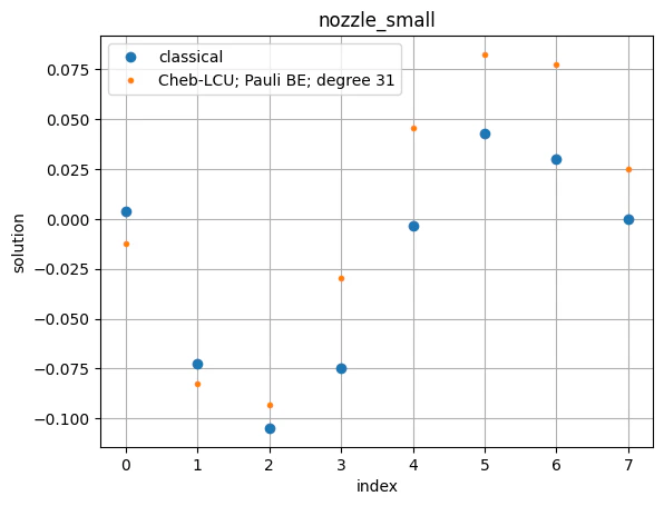
We examine two usecases, starting with a small one, and applying a Pauli-LCU block encoding.
```python theme={null}
mat_small_scr = sparse.load_npz(path / "matrices/nozzle_small_scr.npz")
b_small = np.load(path / "matrices/b_nozzle_small.npy")
print(f"nozzle_small: {mat_small_scr.shape[0]}x{mat_small_scr.shape[1]}")
```
**Output:**
```
nozzle_small: 8x8
```
```python theme={null}
prefs = Preferences()
```
```python theme={null}
qsol_small_pauli, qprog_small_pauli = cheb_lcu_approx_solver(
mat_small_scr,
b_small,
log_poly_degree=4,
be_method="pauli",
preferences=prefs,
constraints=Constraints(optimization_parameter="width"),
)
show(qprog_small_pauli)
```
**Output:**
```
number of Paulis before/after trimming 24/20
Chebyshev LCU size: 4 qubits.
Normalization factor for inversion: 0.7082716135217179
```
**Output:**
```
Submitting job to simulator
```
**Output:**
```
time to syn: 73.70448398590088
```
**Output:**
```
Job: https://platform.classiq.io/jobs/b5381f72-ce8a-470c-b42e-220fb2bfcb12
```
**Output:**
```
time to exe: 17.767388105392456
Quantum program link: https://platform.classiq.io/circuit/3Dt1koIunNqabP53yYwcvdon8Cn
```
We plot the solution vector, and compare to the expected classical result:
```python theme={null}
expected_small = np.linalg.solve(mat_small_scr.toarray(), b_small)
ext_idx = np.argmax(np.abs(expected_small))
correct_sign = np.sign(expected_small[ext_idx]) / np.sign(qsol_small_pauli[ext_idx])
qsol_small_pauli *= correct_sign
plt.plot(expected_small, "o", label="classical")
plt.plot(qsol_small_pauli, ".", label=f"Cheb-LCU; Pauli BE; degree {2*2**4-1}")
plt.title("nozzle_small")
plt.xlabel("index")
plt.ylabel("solution")
plt.legend()
plt.grid(True)
plt.show()
```
 ```python theme={null}
assert np.linalg.norm(qsol_small_pauli - expected_small) < 0.2
```
Next, we move to a larger problem. In a hybrid algorithm, we can relax some of the synthesis preferences to obtain the result a faster (for example, we can set `debug_mode=False` as we can skip the visualization of the quantum program).
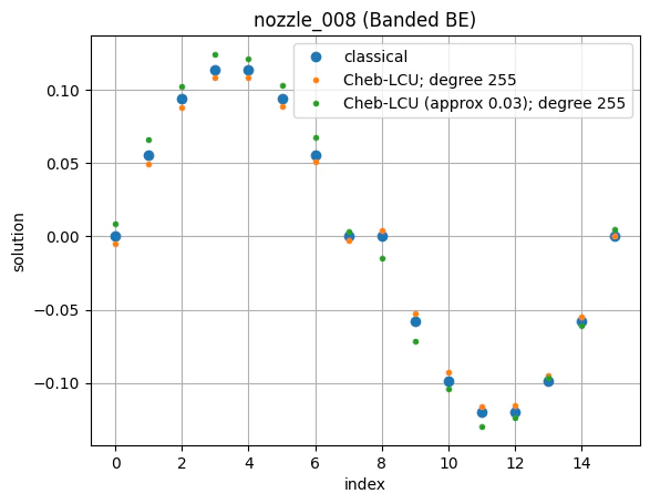
For the larger usecase we work with the Banded Diagonals block-encoding. We compare the approximated version of the solver to the exact one.
```python theme={null}
mat_008_scr = sparse.load_npz(path / "matrices/nozzle_008_mat.npz")
b_008 = np.load(path / "matrices/nozzle_008_b.npy")
print(f"nozzle_008: {mat_008_scr.shape[0]}x{mat_008_scr.shape[1]}")
```
**Output:**
```
nozzle_008: 16x16
```
```python theme={null}
prefs = Preferences(
transpilation_option="none",
optimization_level=0,
debug_mode=False,
qasm3=True,
)
```
```python theme={null}
qsol_008_banded, qprog_008_banded = cheb_lcu_approx_solver(
mat_008_scr,
b_008,
log_poly_degree=7,
be_method="banded",
preferences=prefs,
constraints=Constraints(optimization_parameter="width"),
)
```
**Output:**
```
Chebyshev LCU size: 7 qubits.
Normalization factor for inversion: 0.8180186976736218
```
**Output:**
```
Submitting job to simulator
```
**Output:**
```
time to syn: 48.63558340072632
```
**Output:**
```
Job: https://platform.classiq.io/jobs/3a7ef91e-b24f-4f49-bebb-b7e9fecf2d8e
```
**Output:**
```
time to exe: 70.26255297660828
```
```python theme={null}
SP_APPROX_BOUND = 0.03
qsol_008_banded_approx, qprog_008_banded_approx = cheb_lcu_approx_solver(
mat_008_scr,
b_008,
log_poly_degree=7,
be_method="banded",
approximation=SP_APPROX_BOUND,
preferences=prefs,
constraints=Constraints(optimization_parameter="width"),
)
```
**Output:**
```
linear fit parameters: slope = -0.00010397734302726349, b= 0.014094618961514994
Chebyshev LCU size: 7 qubits.
Normalization factor for inversion: 0.9589833829483215
```
**Output:**
```
Submitting job to simulator
```
**Output:**
```
time to syn: 48.173218727111816
```
**Output:**
```
Job: https://platform.classiq.io/jobs/9ab42c87-977a-4d4f-a5c8-e5841d5c9eaa
```
**Output:**
```
time to exe: 71.8209617137909
```
```python theme={null}
expected_008 = np.linalg.solve(mat_008_scr.toarray(), b_008)
ext_idx = np.argmax(np.abs(expected_008))
correct_sign = np.sign(expected_008[ext_idx]) / np.sign(qsol_008_banded[ext_idx])
qsol_008_banded *= correct_sign
plt.plot(expected_008, "o", label="classical")
plt.plot(qsol_008_banded, ".", label=f"Cheb-LCU; degree {2*2**7-1}")
correct_sign = np.sign(expected_008[ext_idx]) / np.sign(qsol_008_banded_approx[ext_idx])
qsol_008_banded_approx *= correct_sign
plt.plot(
qsol_008_banded_approx,
".",
label=f"Cheb-LCU (approx {SP_APPROX_BOUND}); degree {2*2**7-1}",
)
plt.title("nozzle_008 (Banded BE)")
plt.xlabel("index")
plt.ylabel("solution")
plt.legend()
plt.grid(True)
plt.show()
```
```python theme={null}
assert np.linalg.norm(qsol_small_pauli - expected_small) < 0.2
```
Next, we move to a larger problem. In a hybrid algorithm, we can relax some of the synthesis preferences to obtain the result a faster (for example, we can set `debug_mode=False` as we can skip the visualization of the quantum program).
For the larger usecase we work with the Banded Diagonals block-encoding. We compare the approximated version of the solver to the exact one.
```python theme={null}
mat_008_scr = sparse.load_npz(path / "matrices/nozzle_008_mat.npz")
b_008 = np.load(path / "matrices/nozzle_008_b.npy")
print(f"nozzle_008: {mat_008_scr.shape[0]}x{mat_008_scr.shape[1]}")
```
**Output:**
```
nozzle_008: 16x16
```
```python theme={null}
prefs = Preferences(
transpilation_option="none",
optimization_level=0,
debug_mode=False,
qasm3=True,
)
```
```python theme={null}
qsol_008_banded, qprog_008_banded = cheb_lcu_approx_solver(
mat_008_scr,
b_008,
log_poly_degree=7,
be_method="banded",
preferences=prefs,
constraints=Constraints(optimization_parameter="width"),
)
```
**Output:**
```
Chebyshev LCU size: 7 qubits.
Normalization factor for inversion: 0.8180186976736218
```
**Output:**
```
Submitting job to simulator
```
**Output:**
```
time to syn: 48.63558340072632
```
**Output:**
```
Job: https://platform.classiq.io/jobs/3a7ef91e-b24f-4f49-bebb-b7e9fecf2d8e
```
**Output:**
```
time to exe: 70.26255297660828
```
```python theme={null}
SP_APPROX_BOUND = 0.03
qsol_008_banded_approx, qprog_008_banded_approx = cheb_lcu_approx_solver(
mat_008_scr,
b_008,
log_poly_degree=7,
be_method="banded",
approximation=SP_APPROX_BOUND,
preferences=prefs,
constraints=Constraints(optimization_parameter="width"),
)
```
**Output:**
```
linear fit parameters: slope = -0.00010397734302726349, b= 0.014094618961514994
Chebyshev LCU size: 7 qubits.
Normalization factor for inversion: 0.9589833829483215
```
**Output:**
```
Submitting job to simulator
```
**Output:**
```
time to syn: 48.173218727111816
```
**Output:**
```
Job: https://platform.classiq.io/jobs/9ab42c87-977a-4d4f-a5c8-e5841d5c9eaa
```
**Output:**
```
time to exe: 71.8209617137909
```
```python theme={null}
expected_008 = np.linalg.solve(mat_008_scr.toarray(), b_008)
ext_idx = np.argmax(np.abs(expected_008))
correct_sign = np.sign(expected_008[ext_idx]) / np.sign(qsol_008_banded[ext_idx])
qsol_008_banded *= correct_sign
plt.plot(expected_008, "o", label="classical")
plt.plot(qsol_008_banded, ".", label=f"Cheb-LCU; degree {2*2**7-1}")
correct_sign = np.sign(expected_008[ext_idx]) / np.sign(qsol_008_banded_approx[ext_idx])
qsol_008_banded_approx *= correct_sign
plt.plot(
qsol_008_banded_approx,
".",
label=f"Cheb-LCU (approx {SP_APPROX_BOUND}); degree {2*2**7-1}",
)
plt.title("nozzle_008 (Banded BE)")
plt.xlabel("index")
plt.ylabel("solution")
plt.legend()
plt.grid(True)
plt.show()
```
 ```python theme={null}
assert np.linalg.norm(qsol_008_banded - expected_008) < 0.1
assert np.linalg.norm(qsol_008_banded_approx - expected_008) < 0.1
```
```python theme={null}
assert np.linalg.norm(qsol_008_banded - expected_008) < 0.1
assert np.linalg.norm(qsol_008_banded_approx - expected_008) < 0.1
```