> ## Documentation Index
> Fetch the complete documentation index at: https://docs.classiq.io/llms.txt
> Use this file to discover all available pages before exploring further.
# Hybrid Classical-Quantum Neural Network
Open this notebook in GitHub to run it yourself
## Classical Neural Networks
Neural networks is one of the major branches in machine learning, with wide use in applications and research. A neural network - or, more generally, a deep neural network - is a parametric function of a specific structure (inspired by neural networks in biology), which is trained to capture specific functionality.
In its most basic form, a neural network for learning a function $\vec{f}: \mathbb{R}^N\rightarrow \mathbb{R}^M$ looks as follows:
1. There is an input vector of size $N$ (red circles in Fig. 1).
2. Each entry of the input goes into a hidden layer of size $K$, where each neuron (blue circles in Fig. 1) is defined with an "activation function" $y^{k}(\vec{w}^{(1)}; \vec{x})$ for $k=1,\dots,K$, and $\vec{w}^{(1)}$ are parameters.
3. The output of the hidden layer is sent to the output layer (green circles in Fig. 1) $\tilde{f}^{m}(\vec{w}^{(2)};\vec{y})$ for $m=1,\dots,M$, and $\vec{w}^{(2)}$ are parameters.
The output $\vec{\tilde{f}}$ is thus a parametric function (in $\vec{w}^{(1)},\,\vec{w}^{(2)}$), which can be trained to capture the target function $\vec{f}$.
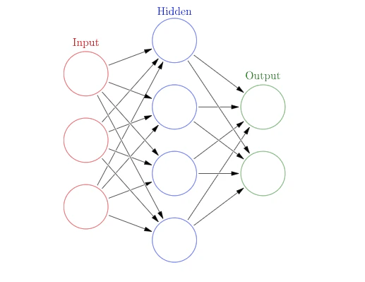 **Deep neural networks** are similar to the description above, having more than one hidden layer.
This provides a more complex structure that can capture more complex functionalities.
## Quantum Neural Networks
The idea of a quantum neural network refers to combining parametric circuits as a replacement for all or some of the classical layers in classical neural networks.
The basic object in QNN is thus a **quantum layer**, which has a classical input and returns a classical output.
The output is obtained by running a quantum program. A quantum layer is thus composed of three parts:
1. A quantum part that encodes the input: This is a parametric quantum function for representing the entries of a single data point.
There are three canonical ways to encode a data vector of size $N$: [angle-encoding](https://github.com/Classiq/classiq-library/blob/main/functions/qmod_library_reference/classiq_open_library/variational_data_encoding/variational_data_encoding.ipynb) using $N$ qubits, [dense angle-encoding](https://github.com/Classiq/classiq-library/blob/main/functions/qmod_library_reference/classiq_open_library/variational_data_encoding/variational_data_encoding.ipynb) using $\lceil N/2\rceil$ qubits, and amplitude-encoding using $\lceil\log_2N\rceil$ qubits.
1. A quantum ansatz part: This is a parametric quantum function, whose parameters are trained as the weights in classical layers.
2. A postprocess classical part, for returning an output classical vector.
The integration of quantum layers in classical neural networks may offer reduction in resources for a given functionality, as the network (or part of it) is expressed via the Hilbert space, providing different expressibility compared to classical networks.
This notebook demonstrates QNN by treating a specific function - the subset majority - for which we construct, train, and verify a hybrid classical-quantum neural network.
The notebook assumes familiarity with Classiq and NN with PyTorch.
See the [QML guide with Classiq](https://github.com/Classiq/classiq-library/blob/main/tutorials/basic_tutorials/qml_with_classiq_guide/qml_with_classiq_guide.ipynb).
## Example: Hybrid Neural Network for the Subset Majority Function
For an integer $N$ and a given subset of indices $S \subset \{0,1,\dots,N\}$ we define the subset majority function, $M_{S}:\{0,1\}^{\times N}\rightarrow \{0,1\}$ that acts on binary strings of size $N$ as follows: it returns 1 if the number of ones within the substring according to $S$ is larger than $|S|//2$, and 0 otherwise,
$$
M_S(\vec{b}) = \left\{ \begin{array}{l l }
1 & \text{if } \sum_{j\in S} b_{j}>|S|//2, \\
0 & \text{otherwise}
\end{array}
\right .
$$
For example, we consider $N=7$ and $S=\{0,1,4\}$:
* The string 0101110 corresponds to the substring 011, for which the number of ones is 2(>1). Therefore, $M_S(0101110)=1$.
* The string 0011111 corresponds to the substring 001, for which the number of ones is 1(=1). Therefore, $M_S(0101110)=0$.
#
## Generating Data for a Specific Example
Let us consider a specific example for our demonstration. We choose $N=10$ and generate all possible data of $2^N$ bit strings. We also take a specific subset $S=\{1, 3, 4, 6, 7, 9\}$.
```python theme={null}
!pip install -qq -U "classiq[qml]"
```
```python theme={null}
import random
import numpy as np
np.random.seed(0)
random.seed(1)
STRING_LEN = 10
majority_data = [
[int(d) for d in np.binary_repr(k, STRING_LEN)] for k in range(2**STRING_LEN)
]
random.shuffle(majority_data) # shuffling the data
```
```python theme={null}
SUBSET_INDICES = [1, 3, 4, 6, 7, 9]
subset_indicator = np.zeros(STRING_LEN)
subset_indicator[SUBSET_INDICES] = 1
```
```python theme={null}
majority = (majority_data @ subset_indicator > len(SUBSET_INDICES) // 2) * 1
labels = [[l] for l in majority]
```
We choose data for training and data for verification, and define the batch size for the corresponding data loaders:
```python theme={null}
TRAINING_SIZE = 340
TEST_SIZE = 512
training_data = majority_data[0:TRAINING_SIZE]
training_labels = labels[0:TRAINING_SIZE]
test_data = majority_data[TRAINING_SIZE : TRAINING_SIZE + TEST_SIZE]
test_labels = labels[TRAINING_SIZE : TRAINING_SIZE + TEST_SIZE]
```
```python theme={null}
BATCH_SIZE = 64
```
```python theme={null}
import numpy as np
import torch
from torch.utils.data import DataLoader, TensorDataset
training_dataset = TensorDataset(
torch.Tensor(training_data), torch.Tensor(training_labels)
) # create dataset
training_dataloader = DataLoader(
training_dataset, batch_size=BATCH_SIZE, shuffle=True, drop_last=False
) # create dataloader
test_dataset = TensorDataset(
torch.Tensor(test_data), torch.Tensor(test_labels)
) # create your dataset
test_dataloader = DataLoader(
test_dataset, batch_size=BATCH_SIZE, shuffle=True, drop_last=False
) # create your dataloader
```
#
## Constructing a Hybrid Network
We build the following hybrid neural network:
**Data flattening $\rightarrow$ A classical linear layer of size 10 to 4 with `Tanh` activation $\rightarrow$ A qlayer of size 4 to 2 $\rightarrow$ a classical linear layer of size 2 to 1 with `ReLU` activation.**
The classical layers can be defined with PyTorch built-in functions.
The quantum layer is constructed with
(1) a [dense angle-encoding](https://github.com/Classiq/classiq-library/blob/main/functions/qmod_library_reference/classiq_open_library/variational_data_encoding/variational_data_encoding.ipynb) function
(2) a simple ansatz with RY and RZZ rotations
(3) a postprocess that is based on a measurement per qubit
#
### The Quantum Layer
```python theme={null}
from classiq import *
from classiq.applications.qnn.types import SavedResult
from classiq.execution import ExecutionPreferences, execute_qnn
@qfunc
def my_ansatz(weights: CArray[CReal], qbv: QArray) -> None:
"""
Gets a quantum variable of $m$ qubits, and applies RY gate on each qubit and RZZ gate on each pair of qubits
in a linear connectivity.
The classical array weights represents the $2m-1$ parametric rotations.
"""
repeat(
count=qbv.len,
iteration=lambda index: RY(weights[index], qbv[index]),
)
repeat(
count=qbv.len - 1,
iteration=lambda index: RZZ(weights[qbv.len + index], qbv[index : index + 2]),
)
```
```python theme={null}
QLAYER_SIZE = 4
num_qubits = int(np.ceil(QLAYER_SIZE / 2))
num_weights = 2 * num_qubits - 1
NUM_SHOTS = 4096
@qfunc
def main(
input_vec: CArray[CReal, QLAYER_SIZE],
weight: CArray[CReal, num_weights],
result: Output[QArray],
) -> None:
"""
The quantum part of the quantum layer.
The prefix for the data loading parameters must be set to `input_` or `i_`.
The prefix for the ansatz parameters must be set to `weights_` or `weight`
"""
encode_on_bloch(input_vec, result)
my_ansatz(weights=weight, qbv=result)
qmod = create_model(
main, execution_preferences=ExecutionPreferences(num_shots=NUM_SHOTS)
)
qprog = synthesize(qmod)
show(qprog)
```
**Output:**
```
Quantum program link: https://platform.classiq.io/circuit/32pQqOSulTv1Qvssd71mPgf4btU
```
```python theme={null}
def my_post_process(result: SavedResult, num_qubits, num_shots) -> torch.Tensor:
"""
Classical postprocess function.
Gets the histogram after execution and returns a vector $\vec{y}$,
where $y_i$ is the probability of measuring 1 on the $i$-th qubit.
"""
res = result.value
yvec = [
(res.counts_of_qubits(k)["1"] if "1" in res.counts_of_qubits(k) else 0)
/ num_shots
for k in range(num_qubits)
]
return torch.tensor(yvec)
```
#
### The Full Hybrid Network
Now, we can define the full network.
```python theme={null}
import torch.nn as nn
from classiq.applications.qnn import QLayer
def create_net(*args, **kwargs) -> nn.Module:
class Net(nn.Module):
def __init__(self, *args, **kwargs):
super().__init__()
self.flatten = nn.Flatten()
self.linear_1 = nn.Linear(STRING_LEN, 4)
self.activation_1 = nn.Tanh()
self.linear_2 = nn.Linear(2, 1)
self.activation_2 = nn.ReLU()
self.qlayer = QLayer(
qprog,
execute_qnn,
post_process=lambda res: my_post_process(
res, num_qubits=num_qubits, num_shots=NUM_SHOTS
),
*args,
**kwargs,
)
def forward(self, x):
x = self.flatten(x)
x = self.linear_1(x)
x = self.activation_1(x)
x = self.qlayer(x) # 4 to 2
x = self.linear_2(x) # 2 to 1
x = self.activation_2(x)
return x
return Net(*args, **kwargs)
my_network = create_net()
```
#
## Training and Verifying the Networks
We define some hyperparameters such as loss function and optimization method, and a training function:
```python theme={null}
import torch.nn as nn
import torch.optim as optim
LEARNING_RATE = 0.05
# choosing our loss function
loss_func = nn.MSELoss()
# choosing our optimizer
optimizer = optim.SGD(my_network.parameters(), lr=LEARNING_RATE)
```
Next, we define a `train` function:
```python theme={null}
import time as time
from torch.utils.data import DataLoader
def train(
network: nn.Module,
data_loader: DataLoader,
loss_func: nn.modules.loss._Loss,
optimizer: optim.Optimizer,
epoch: int = 20,
) -> None:
for index in range(epoch):
start = time.time()
for data, label in data_loader:
optimizer.zero_grad()
output = network(data)
loss = loss_func(output, label.type(output.dtype))
loss.backward()
optimizer.step()
print(index, f"\tloss = {loss.item()}", "time", time.time() - start)
```
We also define a validation function, `check_accuracy`, which tests a trained network on new data:
```python theme={null}
from torch import Tensor
def get_correctly_guessed_labels_function(
model: nn.Module, data: Tensor, labels: Tensor
) -> int:
predictions = model(data)
list_of_predictions = [
round(prediction.type(torch.float).item()) for prediction in predictions
]
correct = sum(
[
list_of_predictions[k] == labels.flatten().tolist()[k]
for k in range(len(predictions))
]
)
return correct
def _get_amount_of_labels(labels: Tensor) -> int:
# the first dimension of `labels` is `batch_size`
return labels.size(0)
def check_accuracy(
network: nn.Module,
data_loader: DataLoader,
should_print: bool = True,
) -> float:
num_correct = 0
total = 0
network.eval()
with torch.no_grad():
for data, labels in data_loader:
num_correct += get_correctly_guessed_labels_function(network, data, labels)
total += _get_amount_of_labels(labels)
accuracy = float(num_correct) / float(total)
if should_print:
print(f"Test accuracy of the model: {accuracy*100:.2f}%")
print(f"num correct: {num_correct}, total: {total}")
return accuracy
```
#
## Training and Verifying the Network
For convenience, we load a pre-trained model and set the epoch size to
1. Training a network takes around 30 epochs.
```python theme={null}
# comment out for training
my_network.load_state_dict(torch.load("trained_model.pth"))
num_epoch = 1
# uncomment out for training
# epoch=30
```
```python theme={null}
data_loader = training_dataloader
train(my_network, training_dataloader, loss_func, optimizer, epoch=num_epoch)
```
**Output:**
```
0 loss = 0.09676678478717804 time 169.12708473205566
```
```python theme={null}
accuracy = check_accuracy(my_network, test_dataloader)
```
**Output:**
```
Test accuracy of the model: 97.07%
num correct: 497, total: 512
```
**Deep neural networks** are similar to the description above, having more than one hidden layer.
This provides a more complex structure that can capture more complex functionalities.
## Quantum Neural Networks
The idea of a quantum neural network refers to combining parametric circuits as a replacement for all or some of the classical layers in classical neural networks.
The basic object in QNN is thus a **quantum layer**, which has a classical input and returns a classical output.
The output is obtained by running a quantum program. A quantum layer is thus composed of three parts:
1. A quantum part that encodes the input: This is a parametric quantum function for representing the entries of a single data point.
There are three canonical ways to encode a data vector of size $N$: [angle-encoding](https://github.com/Classiq/classiq-library/blob/main/functions/qmod_library_reference/classiq_open_library/variational_data_encoding/variational_data_encoding.ipynb) using $N$ qubits, [dense angle-encoding](https://github.com/Classiq/classiq-library/blob/main/functions/qmod_library_reference/classiq_open_library/variational_data_encoding/variational_data_encoding.ipynb) using $\lceil N/2\rceil$ qubits, and amplitude-encoding using $\lceil\log_2N\rceil$ qubits.
1. A quantum ansatz part: This is a parametric quantum function, whose parameters are trained as the weights in classical layers.
2. A postprocess classical part, for returning an output classical vector.
The integration of quantum layers in classical neural networks may offer reduction in resources for a given functionality, as the network (or part of it) is expressed via the Hilbert space, providing different expressibility compared to classical networks.
This notebook demonstrates QNN by treating a specific function - the subset majority - for which we construct, train, and verify a hybrid classical-quantum neural network.
The notebook assumes familiarity with Classiq and NN with PyTorch.
See the [QML guide with Classiq](https://github.com/Classiq/classiq-library/blob/main/tutorials/basic_tutorials/qml_with_classiq_guide/qml_with_classiq_guide.ipynb).
## Example: Hybrid Neural Network for the Subset Majority Function
For an integer $N$ and a given subset of indices $S \subset \{0,1,\dots,N\}$ we define the subset majority function, $M_{S}:\{0,1\}^{\times N}\rightarrow \{0,1\}$ that acts on binary strings of size $N$ as follows: it returns 1 if the number of ones within the substring according to $S$ is larger than $|S|//2$, and 0 otherwise,
$$
M_S(\vec{b}) = \left\{ \begin{array}{l l }
1 & \text{if } \sum_{j\in S} b_{j}>|S|//2, \\
0 & \text{otherwise}
\end{array}
\right .
$$
For example, we consider $N=7$ and $S=\{0,1,4\}$:
* The string 0101110 corresponds to the substring 011, for which the number of ones is 2(>1). Therefore, $M_S(0101110)=1$.
* The string 0011111 corresponds to the substring 001, for which the number of ones is 1(=1). Therefore, $M_S(0101110)=0$.
#
## Generating Data for a Specific Example
Let us consider a specific example for our demonstration. We choose $N=10$ and generate all possible data of $2^N$ bit strings. We also take a specific subset $S=\{1, 3, 4, 6, 7, 9\}$.
```python theme={null}
!pip install -qq -U "classiq[qml]"
```
```python theme={null}
import random
import numpy as np
np.random.seed(0)
random.seed(1)
STRING_LEN = 10
majority_data = [
[int(d) for d in np.binary_repr(k, STRING_LEN)] for k in range(2**STRING_LEN)
]
random.shuffle(majority_data) # shuffling the data
```
```python theme={null}
SUBSET_INDICES = [1, 3, 4, 6, 7, 9]
subset_indicator = np.zeros(STRING_LEN)
subset_indicator[SUBSET_INDICES] = 1
```
```python theme={null}
majority = (majority_data @ subset_indicator > len(SUBSET_INDICES) // 2) * 1
labels = [[l] for l in majority]
```
We choose data for training and data for verification, and define the batch size for the corresponding data loaders:
```python theme={null}
TRAINING_SIZE = 340
TEST_SIZE = 512
training_data = majority_data[0:TRAINING_SIZE]
training_labels = labels[0:TRAINING_SIZE]
test_data = majority_data[TRAINING_SIZE : TRAINING_SIZE + TEST_SIZE]
test_labels = labels[TRAINING_SIZE : TRAINING_SIZE + TEST_SIZE]
```
```python theme={null}
BATCH_SIZE = 64
```
```python theme={null}
import numpy as np
import torch
from torch.utils.data import DataLoader, TensorDataset
training_dataset = TensorDataset(
torch.Tensor(training_data), torch.Tensor(training_labels)
) # create dataset
training_dataloader = DataLoader(
training_dataset, batch_size=BATCH_SIZE, shuffle=True, drop_last=False
) # create dataloader
test_dataset = TensorDataset(
torch.Tensor(test_data), torch.Tensor(test_labels)
) # create your dataset
test_dataloader = DataLoader(
test_dataset, batch_size=BATCH_SIZE, shuffle=True, drop_last=False
) # create your dataloader
```
#
## Constructing a Hybrid Network
We build the following hybrid neural network:
**Data flattening $\rightarrow$ A classical linear layer of size 10 to 4 with `Tanh` activation $\rightarrow$ A qlayer of size 4 to 2 $\rightarrow$ a classical linear layer of size 2 to 1 with `ReLU` activation.**
The classical layers can be defined with PyTorch built-in functions.
The quantum layer is constructed with
(1) a [dense angle-encoding](https://github.com/Classiq/classiq-library/blob/main/functions/qmod_library_reference/classiq_open_library/variational_data_encoding/variational_data_encoding.ipynb) function
(2) a simple ansatz with RY and RZZ rotations
(3) a postprocess that is based on a measurement per qubit
#
### The Quantum Layer
```python theme={null}
from classiq import *
from classiq.applications.qnn.types import SavedResult
from classiq.execution import ExecutionPreferences, execute_qnn
@qfunc
def my_ansatz(weights: CArray[CReal], qbv: QArray) -> None:
"""
Gets a quantum variable of $m$ qubits, and applies RY gate on each qubit and RZZ gate on each pair of qubits
in a linear connectivity.
The classical array weights represents the $2m-1$ parametric rotations.
"""
repeat(
count=qbv.len,
iteration=lambda index: RY(weights[index], qbv[index]),
)
repeat(
count=qbv.len - 1,
iteration=lambda index: RZZ(weights[qbv.len + index], qbv[index : index + 2]),
)
```
```python theme={null}
QLAYER_SIZE = 4
num_qubits = int(np.ceil(QLAYER_SIZE / 2))
num_weights = 2 * num_qubits - 1
NUM_SHOTS = 4096
@qfunc
def main(
input_vec: CArray[CReal, QLAYER_SIZE],
weight: CArray[CReal, num_weights],
result: Output[QArray],
) -> None:
"""
The quantum part of the quantum layer.
The prefix for the data loading parameters must be set to `input_` or `i_`.
The prefix for the ansatz parameters must be set to `weights_` or `weight`
"""
encode_on_bloch(input_vec, result)
my_ansatz(weights=weight, qbv=result)
qmod = create_model(
main, execution_preferences=ExecutionPreferences(num_shots=NUM_SHOTS)
)
qprog = synthesize(qmod)
show(qprog)
```
**Output:**
```
Quantum program link: https://platform.classiq.io/circuit/32pQqOSulTv1Qvssd71mPgf4btU
```
```python theme={null}
def my_post_process(result: SavedResult, num_qubits, num_shots) -> torch.Tensor:
"""
Classical postprocess function.
Gets the histogram after execution and returns a vector $\vec{y}$,
where $y_i$ is the probability of measuring 1 on the $i$-th qubit.
"""
res = result.value
yvec = [
(res.counts_of_qubits(k)["1"] if "1" in res.counts_of_qubits(k) else 0)
/ num_shots
for k in range(num_qubits)
]
return torch.tensor(yvec)
```
#
### The Full Hybrid Network
Now, we can define the full network.
```python theme={null}
import torch.nn as nn
from classiq.applications.qnn import QLayer
def create_net(*args, **kwargs) -> nn.Module:
class Net(nn.Module):
def __init__(self, *args, **kwargs):
super().__init__()
self.flatten = nn.Flatten()
self.linear_1 = nn.Linear(STRING_LEN, 4)
self.activation_1 = nn.Tanh()
self.linear_2 = nn.Linear(2, 1)
self.activation_2 = nn.ReLU()
self.qlayer = QLayer(
qprog,
execute_qnn,
post_process=lambda res: my_post_process(
res, num_qubits=num_qubits, num_shots=NUM_SHOTS
),
*args,
**kwargs,
)
def forward(self, x):
x = self.flatten(x)
x = self.linear_1(x)
x = self.activation_1(x)
x = self.qlayer(x) # 4 to 2
x = self.linear_2(x) # 2 to 1
x = self.activation_2(x)
return x
return Net(*args, **kwargs)
my_network = create_net()
```
#
## Training and Verifying the Networks
We define some hyperparameters such as loss function and optimization method, and a training function:
```python theme={null}
import torch.nn as nn
import torch.optim as optim
LEARNING_RATE = 0.05
# choosing our loss function
loss_func = nn.MSELoss()
# choosing our optimizer
optimizer = optim.SGD(my_network.parameters(), lr=LEARNING_RATE)
```
Next, we define a `train` function:
```python theme={null}
import time as time
from torch.utils.data import DataLoader
def train(
network: nn.Module,
data_loader: DataLoader,
loss_func: nn.modules.loss._Loss,
optimizer: optim.Optimizer,
epoch: int = 20,
) -> None:
for index in range(epoch):
start = time.time()
for data, label in data_loader:
optimizer.zero_grad()
output = network(data)
loss = loss_func(output, label.type(output.dtype))
loss.backward()
optimizer.step()
print(index, f"\tloss = {loss.item()}", "time", time.time() - start)
```
We also define a validation function, `check_accuracy`, which tests a trained network on new data:
```python theme={null}
from torch import Tensor
def get_correctly_guessed_labels_function(
model: nn.Module, data: Tensor, labels: Tensor
) -> int:
predictions = model(data)
list_of_predictions = [
round(prediction.type(torch.float).item()) for prediction in predictions
]
correct = sum(
[
list_of_predictions[k] == labels.flatten().tolist()[k]
for k in range(len(predictions))
]
)
return correct
def _get_amount_of_labels(labels: Tensor) -> int:
# the first dimension of `labels` is `batch_size`
return labels.size(0)
def check_accuracy(
network: nn.Module,
data_loader: DataLoader,
should_print: bool = True,
) -> float:
num_correct = 0
total = 0
network.eval()
with torch.no_grad():
for data, labels in data_loader:
num_correct += get_correctly_guessed_labels_function(network, data, labels)
total += _get_amount_of_labels(labels)
accuracy = float(num_correct) / float(total)
if should_print:
print(f"Test accuracy of the model: {accuracy*100:.2f}%")
print(f"num correct: {num_correct}, total: {total}")
return accuracy
```
#
## Training and Verifying the Network
For convenience, we load a pre-trained model and set the epoch size to
1. Training a network takes around 30 epochs.
```python theme={null}
# comment out for training
my_network.load_state_dict(torch.load("trained_model.pth"))
num_epoch = 1
# uncomment out for training
# epoch=30
```
```python theme={null}
data_loader = training_dataloader
train(my_network, training_dataloader, loss_func, optimizer, epoch=num_epoch)
```
**Output:**
```
0 loss = 0.09676678478717804 time 169.12708473205566
```
```python theme={null}
accuracy = check_accuracy(my_network, test_dataloader)
```
**Output:**
```
Test accuracy of the model: 97.07%
num correct: 497, total: 512
```